Vision Encoders: How Machines Learned to See — From Convolutions to Vision Transformers

Understanding the two paradigms of visual representation learning — from local feature extraction with CNNs to global attention with Vision Transformers.

What Does It Mean to "See"?

Let us start with a simple thought experiment. Imagine you are reading a page from a book. Your eyes move word by word, left to right, top to bottom. You process small chunks of text at a time, and your brain builds understanding from these local pieces.

Now imagine you are looking at a photograph of a beach. You do not scan it word by word. Instead, you take in the entire scene at once — the ocean, the sand, the person walking, the seagull in the sky. You understand the relationships between distant objects instantly: the seagull is above the water, the person is on the sand.

These two modes of perception — local, sequential processing versus global, holistic understanding — turn out to be exactly the two paradigms that define how neural networks learn to "see."

The first paradigm is the Convolutional Neural Network (CNN), which processes images through small local filters that slide across the image — much like reading word by word. The second paradigm is the Vision Transformer (ViT), which processes the entire image at once by treating it as a sequence of patches and computing attention between all of them — much like taking in a photograph holistically.

But before we can compare them, we need to understand how each one works. This brings us to the fundamental operation behind CNNs: the convolution.

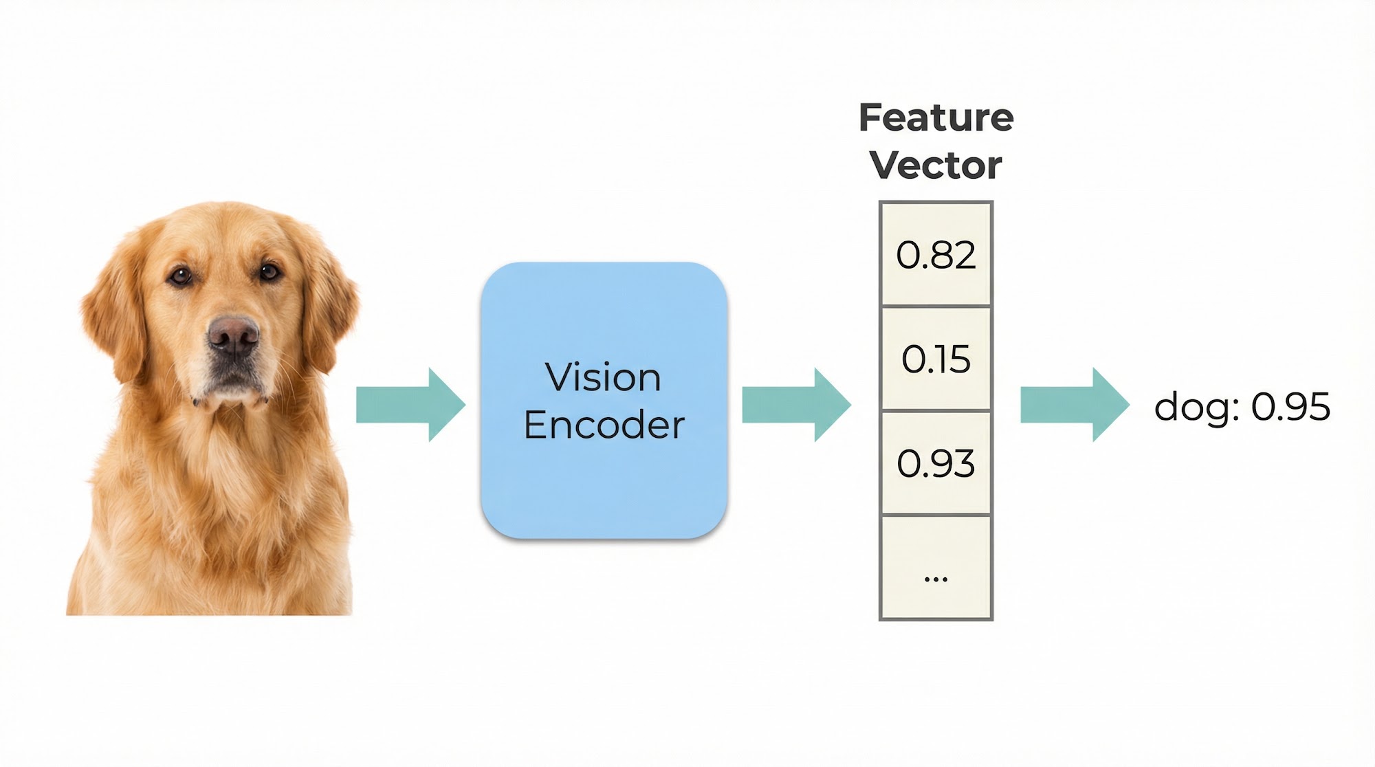
A vision encoder converts raw pixels into a compact feature representation.

The Convolution Operation — Learning Local Patterns

Let us think of a convolution as a magnifying glass that you slide across a photograph. At each position, you look at a small patch of pixels, perform a calculation, and write down a single number. When you have slid the magnifying glass across the entire image, you have a new grid of numbers — a feature map — that captures some local pattern from the original image.

Mathematically, a 2D convolution takes an input image $I$ and a small filter (also called a kernel) $K$ of size $k \times k$ , and computes the output feature map $O$ as follows:

O(i, j) = \sum_{m=0}^{k-1} \sum_{n=0}^{k-1} I(i+m, j+n) \cdot K(m, n)

This looks intimidating, but it is simply a weighted sum of the pixel values in a local neighborhood. Let us plug in some simple numbers to see how this works.

Suppose we have a small 4x4 image and a 3x3 filter:

Image (4x4):

Filter (3x3):

1  0  1
0  1  0
1  0  1

To compute the output at position (0,0), we overlay the 3x3 filter on the top-left corner of the image and compute the element-wise product, then sum:

O(0,0) = (1 \times 1) + (2 \times 0) + (3 \times 1) + (0 \times 0) + (1 \times 1) + (2 \times 0) + (1 \times 1) + (0 \times 0) + (1 \times 1) = 1 + 0 + 3 + 0 + 1 + 0 + 1 + 0 + 1 = 7

We repeat this at every valid position, sliding the filter across the image. This is exactly what we want — a single operation that summarizes a local region of the image into one number.

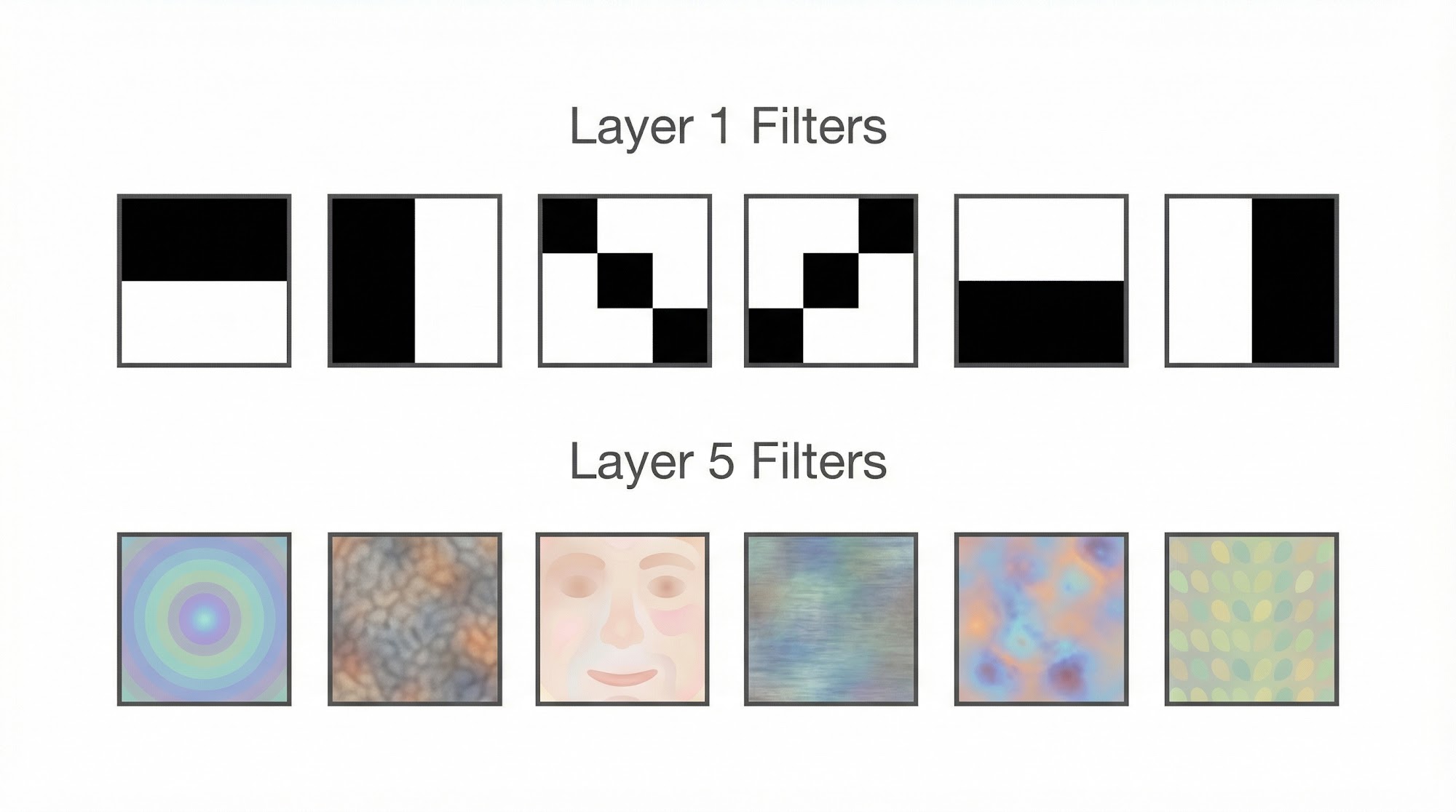
But here is the key insight: the filter values are learnable. During training, the neural network discovers which local patterns are important. Early layers tend to learn simple patterns like edges and corners. Deeper layers learn more complex patterns like textures, object parts, and eventually entire objects.

A convolution filter slides across the image, computing a weighted sum at each position.

Early layers detect edges; deeper layers recognize complex visual patterns.

Building a CNN — Stacking Convolutions

Now that we understand how a single convolution works, let us see what happens when we stack multiple convolutional layers together.

The idea is beautifully simple: each layer captures progressively higher-level features. The first layer might detect edges. The second layer combines edges into textures. The third layer combines textures into object parts. And the final layers recognize entire objects.

Between convolution layers, we typically apply two operations:

ReLU activation — which simply sets all negative values to zero. This introduces non-linearity, allowing the network to learn complex patterns.
Max Pooling — which shrinks the spatial dimensions by keeping only the maximum value in each local region.

The max pooling operation over a 2x2 window can be written as:

\text{MaxPool}(i, j) = \max \big( O(2i, 2j),\; O(2i+1, 2j),\; O(2i, 2j+1),\; O(2i+1, 2j+1) \big)

Let us plug in some simple numbers. Suppose we have a 4x4 feature map:

With a 2x2 max pooling window and stride 2, we divide the feature map into four 2x2 blocks and take the maximum of each:

Top-left block: max(6, 2, 1, 7) = 7
Top-right block: max(3, 1, 0, 4) = 4
Bottom-left block: max(8, 0, 3, 1) = 8
Bottom-right block: max(5, 2, 2, 9) = 9

The output is a 2x2 feature map: [[7, 4], [8, 9]]. We have reduced the spatial resolution by half while keeping the most prominent features. This is exactly what we want.

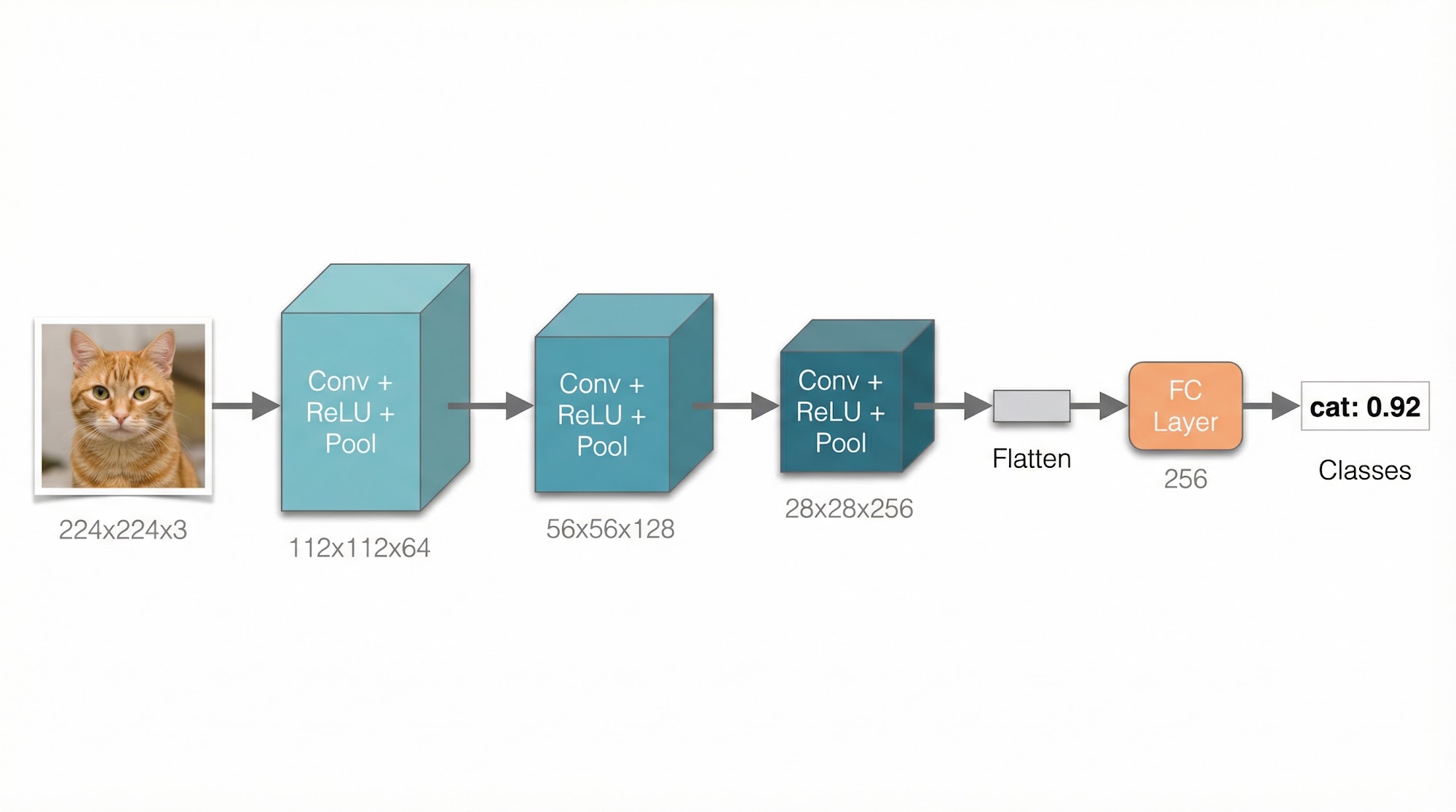
The overall CNN pipeline looks like this: an image flows through several blocks of convolution + ReLU + pooling, and the spatial dimensions shrink while the number of feature channels grows. Finally, the features are flattened and passed through a fully connected layer for classification.

A CNN progressively extracts higher-level features through stacked convolutions.

Here is a minimal CNN implementation in PyTorch:

import torch
import torch.nn as nn

class SimpleCNN(nn.Module):
    def __init__(self, num_classes=10):
        super().__init__()
        self.features = nn.Sequential(
            nn.Conv2d(3, 32, kernel_size=3, padding=1),
            nn.ReLU(),
            nn.MaxPool2d(2),
            nn.Conv2d(32, 64, kernel_size=3, padding=1),
            nn.ReLU(),
            nn.MaxPool2d(2),
            nn.Conv2d(64, 128, kernel_size=3, padding=1),
            nn.ReLU(),
            nn.MaxPool2d(2),
        )
        self.classifier = nn.Sequential(
            nn.Flatten(),
            nn.Linear(128 * 4 * 4, 256),
            nn.ReLU(),
            nn.Linear(256, num_classes),
        )

    def forward(self, x):
        x = self.features(x)
        x = self.classifier(x)
        return x

Let us understand this code. We define three convolutional blocks, each with a 3x3 convolution, ReLU activation, and 2x2 max pooling. The number of channels increases from 3 (RGB input) to 32, then 64, then 128. After the convolutional layers, we flatten the features and pass them through two fully connected layers to produce class predictions.

This architecture follows the lineage of landmark models like LeNet (1998), AlexNet (2012), VGG (2014), and ResNet (2015). Each advanced the state of the art by going deeper — from 5 layers to 152 layers — but they all relied on the same fundamental operation: the convolution.

The Limitation of Locality — Why CNNs Struggle with Global Context

Now, you might be thinking: if CNNs are so powerful, why do we need anything else?

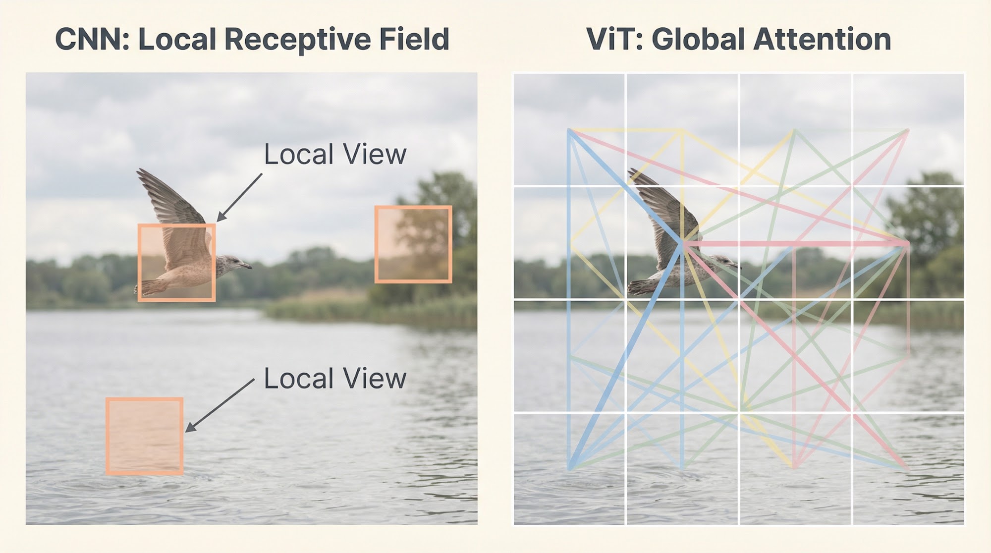
The answer lies in a fundamental limitation called the receptive field problem. Each convolution filter only looks at a small local neighborhood — typically 3x3 or 5x5 pixels. The output neuron at any position only "knows" about the pixels in that tiny window.

Of course, as you stack more layers, the receptive field grows — a neuron in the fifth layer indirectly sees a much larger region of the original image. But this comes at a cost:

Information must pass through many layers to travel from one part of the image to another. A relationship between a bird in the top-left corner and the water in the bottom-right corner requires the signal to propagate through dozens of layers.
Stacking more layers is expensive — it requires more parameters, more computation, and more memory. It also introduces problems like vanishing gradients, which make training difficult.
Long-range dependencies are learned indirectly. The network must learn to route information through many intermediate representations, which is inefficient and unreliable.

But what if a network could look at the entire image at once? What if every part of the image could directly communicate with every other part in a single operation?

This is precisely the idea behind the Vision Transformer.

CNNs see locally; Transformers attend to the entire image at once.

From Images to Sequences — Patch Embeddings

In 2020, a paper from Google Research changed everything. Titled "An Image is Worth 16x16 Words," it introduced the Vision Transformer (ViT) — and the key insight was remarkably simple.

Instead of applying convolutions to an image, split the image into fixed-size patches and treat each patch as a "word." Then apply the standard Transformer architecture — the same one used for natural language processing — to this sequence of patch tokens.

Let us think of it as a jigsaw puzzle. You take a photograph, cut it into 16x16-pixel squares, and lay them out in a row. Each piece becomes a token, just like a word in a sentence. The Transformer then processes these tokens, allowing every patch to attend to every other patch.

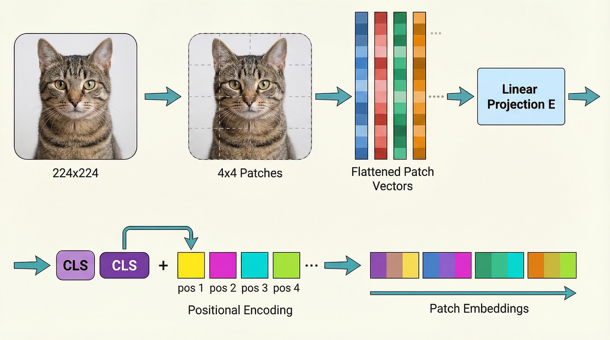
Concretely, here is how it works. Given an image of size $H \times W$ with $C$ channels and a patch size of $P \times P$ :

Divide the image into $N = \frac{H \times W}{P^2}$ non-overlapping patches
Flatten each patch into a vector of size $P^2 \times C$
Linearly project each flattened patch into a $D$ -dimensional embedding

The patch embedding is computed as:

\mathbf{z}_i = \mathbf{E} \cdot \mathbf{x}_i^{\text{patch}} + \mathbf{e}_i^{\text{pos}}, \quad i = 1, \ldots, N

where $\mathbf{E} \in \mathbb{R}^{D \times (P^2 C)}$ is the projection matrix, $\mathbf{x}_i^{\text{patch}}$ is the flattened patch, and $\mathbf{e}_i^{\text{pos}}$ is the positional embedding for the $i$ -th patch.

Let us plug in some numbers. For a standard 224x224 RGB image with patch size 16:

Each patch has size: $16 \times 16 \times 3 = 768$ values
Number of patches: $\frac{224 \times 224}{16 \times 16} = \frac{50176}{256} = 196$ patches
Each patch is projected to dimension $D = 768$

So the image becomes a sequence of 196 tokens, each of dimension 768. This is very similar to how a sentence of 196 words would be represented — each word as a 768-dimensional embedding.

A special [CLS] token is prepended to the sequence. This token aggregates global information from all patches through self-attention and is used for classification.

Finally, positional embeddings are added so the model knows the spatial arrangement of the patches. Without them, the model would have no way of knowing which patch came from the top-left versus the bottom-right.

An image is split into patches, each projected into an embedding — just like words in a sentence.

Self-Attention — How Patches Talk to Each Other

Now we have our image represented as a sequence of patch tokens. The next question is: how do these patches communicate with each other?

This brings us to self-attention — the core mechanism of the Transformer. Let us build intuition with an analogy.

Imagine a team meeting with 5 people seated around a table. When person A is speaking, they look around the table and decide how much to pay attention to each other person. Maybe person B said something highly relevant, so A pays a lot of attention to B. Person C said something unrelated, so A mostly ignores C.

In self-attention, every patch does exactly this. Each patch "asks" every other patch: "How relevant are you to me?" Based on the answers, it computes a weighted combination of information from all patches.

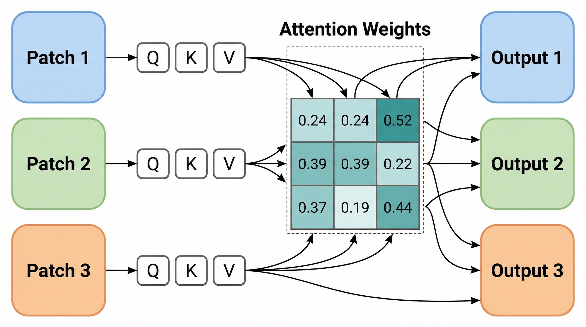
Formally, each patch embedding is projected into three vectors:

Query (Q) — "What am I looking for?"
Key (K) — "What information do I have?"
Value (V) — "What information will I share?"

The attention is computed as:

\text{Attention}(Q, K, V) = \text{softmax}\!\left(\frac{QK^T}{\sqrt{d_k}}\right) V

Let us plug in some simple numbers to see how this works. Suppose we have just 3 patches, each with 4-dimensional embeddings. After projecting to Q, K, V (assume $d_k = 4$ ):

Q = \begin{bmatrix} 1 & 0 & 1 & 0 \\ 0 & 1 & 0 & 1 \\ 1 & 1 & 0 & 0 \end{bmatrix}, \quad K = \begin{bmatrix} 1 & 1 & 0 & 0 \\ 0 & 0 & 1 & 1 \\ 1 & 0 & 1 & 0 \end{bmatrix}

Step 1: Compute $QK^T$ (dot product of queries with keys):

QK^T = \begin{bmatrix} 1 & 1 & 2 \\ 1 & 1 & 0 \\ 1 & 0 & 1 \end{bmatrix}

Step 2: Scale by $\frac{1}{\sqrt{d_k}} = \frac{1}{\sqrt{4}} = 0.5$ :

\frac{QK^T}{\sqrt{d_k}} = \begin{bmatrix} 0.5 & 0.5 & 1.0 \\ 0.5 & 0.5 & 0 \\ 0.5 & 0 & 0.5 \end{bmatrix}

Step 3: Apply softmax row-wise to get attention weights. For the first row: $\text{softmax}([0.5, 0.5, 1.0]) \approx [0.24, 0.24, 0.52]$ .

This tells us that patch 1 pays the most attention to patch 3 (weight 0.52), and equal attention to patches 1 and 2. This is exactly what we want — the attention mechanism automatically determines which patches are most relevant to each other.

Step 4: Multiply the attention weights by V to get the output — a weighted combination of values.

In a Vision Transformer, we use multi-head attention, which simply runs this process multiple times in parallel with different projection weights. Each "head" can learn to attend to different types of relationships — one head might learn spatial proximity, another might learn color similarity, another might learn semantic relationships.

Each patch computes attention scores to decide which other patches to focus on.

The Vision Transformer Architecture

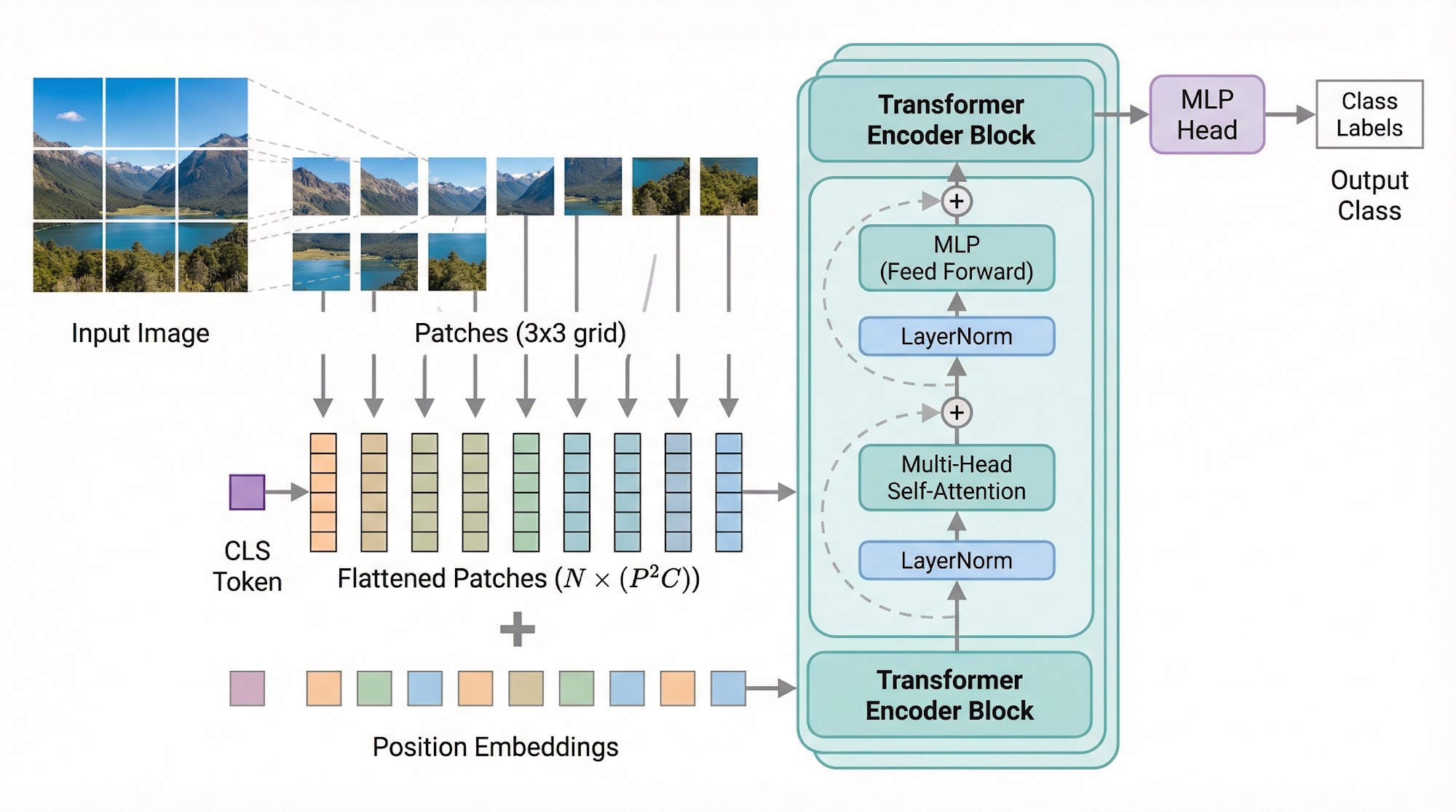
Now we have all the pieces of the puzzle ready. Let us assemble the full Vision Transformer.

The architecture is surprisingly elegant:

Patch Embedding Layer — Split the image into patches and project them
Prepend [CLS] Token — Add a learnable classification token
Add Positional Embeddings — Encode spatial information
Transformer Encoder Blocks — Stack $L$ $L$ identical blocks, each containing:
- Layer Normalization
- Multi-Head Self-Attention (with residual connection)
- Layer Normalization
- MLP (two linear layers with GELU activation, with residual connection)
Classification Head — Take the [CLS] token output and pass through an MLP for prediction

Each Transformer encoder block can be written as:

\mathbf{z}'_l = \text{MSA}(\text{LN}(\mathbf{z}_{l-1})) + \mathbf{z}_{l-1}

\mathbf{z}_l = \text{MLP}(\text{LN}(\mathbf{z}'_l)) + \mathbf{z}'_l

where MSA is multi-head self-attention, LN is layer normalization, and MLP is a two-layer feedforward network.

The original ViT paper (Dosovitskiy et al., 2020) showed a remarkable result: when trained on sufficient data (the JFT-300M dataset with 300 million images), ViT-Large surpassed the best CNNs on ImageNet while requiring fewer computational resources to train. However, when trained on smaller datasets like ImageNet alone (1.2M images), ViT performed worse than CNNs. This is because CNNs have built-in inductive biases — translation equivariance and locality — that help them learn efficiently from limited data. ViTs must learn these patterns from scratch, which requires more data.

The Vision Transformer processes image patches through Transformer encoder blocks.

Here is a minimal ViT implementation in PyTorch:

import torch
import torch.nn as nn

class PatchEmbedding(nn.Module):
    def __init__(self, img_size=32, patch_size=4, in_channels=3, embed_dim=128):
        super().__init__()
        self.num_patches = (img_size // patch_size) ** 2
        self.proj = nn.Conv2d(in_channels, embed_dim,
                              kernel_size=patch_size, stride=patch_size)

    def forward(self, x):
        # x: (B, C, H, W) -> (B, embed_dim, H/P, W/P)
        x = self.proj(x)
        # Flatten spatial dims: (B, embed_dim, N) -> (B, N, embed_dim)
        x = x.flatten(2).transpose(1, 2)
        return x

class SimpleViT(nn.Module):
    def __init__(self, img_size=32, patch_size=4, in_channels=3,
                 embed_dim=128, num_heads=4, num_layers=4, num_classes=10):
        super().__init__()
        self.patch_embed = PatchEmbedding(img_size, patch_size,
                                          in_channels, embed_dim)
        num_patches = (img_size // patch_size) ** 2
        # Learnable [CLS] token and positional embeddings
        self.cls_token = nn.Parameter(torch.zeros(1, 1, embed_dim))
        self.pos_embed = nn.Parameter(
            torch.randn(1, num_patches + 1, embed_dim) * 0.02)
        # Transformer encoder
        encoder_layer = nn.TransformerEncoderLayer(
            d_model=embed_dim, nhead=num_heads,
            dim_feedforward=embed_dim * 4, activation='gelu',
            batch_first=True, norm_first=True)
        self.transformer = nn.TransformerEncoder(
            encoder_layer, num_layers=num_layers)
        # Classification head
        self.head = nn.Linear(embed_dim, num_classes)

    def forward(self, x):
        B = x.shape[0]
        x = self.patch_embed(x)
        cls = self.cls_token.expand(B, -1, -1)
        x = torch.cat([cls, x], dim=1)
        x = x + self.pos_embed
        x = self.transformer(x)
        return self.head(x[:, 0])  # CLS token output

Let us understand this code. The PatchEmbedding module uses a convolution with kernel_size=patch_size and stride=patch_size to split the image into non-overlapping patches and project each into an embedding — this is equivalent to the linear projection we described earlier, but more efficient. The SimpleViT module prepends a [CLS] token, adds positional embeddings, passes everything through a stack of Transformer encoder layers, and uses the [CLS] token output for classification.

CNNs vs. Vision Transformers — When to Use What

Now that we understand both architectures, the natural question is: which one should I use?

The answer depends on your data, your compute budget, and your problem.

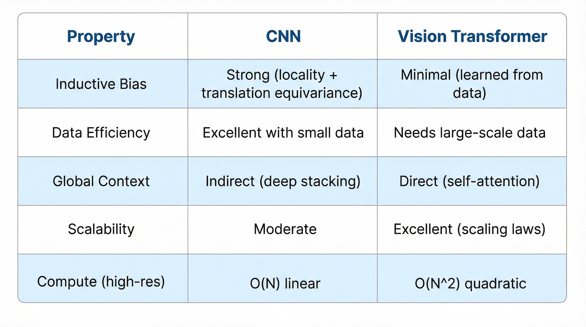
Inductive biases. CNNs have strong built-in assumptions: translation equivariance (a cat in the top-left corner is processed the same way as a cat in the bottom-right) and locality (nearby pixels are more related than distant ones). These are powerful priors that help CNNs learn efficiently from small datasets. ViTs have almost no built-in assumptions — they must learn spatial relationships entirely from data.

Data efficiency. On small datasets (a few thousand images), CNNs consistently outperform ViTs. The inductive biases act as a form of regularization. However, on large datasets (millions of images), ViTs overtake CNNs because they are not limited by those same biases — they can discover patterns that CNNs cannot express.

Scalability. ViTs scale better with increasing model size and data. The Transformer architecture has proven to follow reliable scaling laws — more parameters and more data consistently lead to better performance. This is the same phenomenon we see in large language models.

Computational cost. Self-attention has quadratic complexity in the number of patches ( $O(N^2)$ ), while convolutions are linear in the number of pixels. For high-resolution images, this matters. However, many optimizations exist (windowed attention, linear attention, etc.).

Hybrid approaches. Modern architectures increasingly combine the best of both worlds. Models like CoAtNet use CNN stems for early layers (where locality matters most) and Transformer blocks for later layers (where global context is valuable). DeiT (Data-efficient Image Transformers) introduced distillation from a CNN teacher, allowing ViTs to train effectively on ImageNet alone.

CNNs and ViTs excel in different regimes — the choice depends on data and compute.

Practical Implementation — Training a ViT on CIFAR-10

Enough theory, let us look at some practical implementation now. We will train our SimpleViT on the CIFAR-10 dataset, which contains 60,000 32x32 color images across 10 classes.

import torchvision
import torchvision.transforms as transforms

# Data loading with augmentation
transform_train = transforms.Compose([
    transforms.RandomCrop(32, padding=4),
    transforms.RandomHorizontalFlip(),
    transforms.ToTensor(),
    transforms.Normalize((0.4914, 0.4822, 0.4465),
                         (0.2023, 0.1994, 0.2010)),
])

trainset = torchvision.datasets.CIFAR10(root='./data', train=True,
                                         download=True, transform=transform_train)
trainloader = torch.utils.data.DataLoader(trainset, batch_size=128,
                                           shuffle=True, num_workers=2)

# Initialize model, loss, optimizer
model = SimpleViT(img_size=32, patch_size=4, embed_dim=128,
                  num_heads=4, num_layers=4, num_classes=10).cuda()
criterion = nn.CrossEntropyLoss()
optimizer = torch.optim.AdamW(model.parameters(), lr=3e-4,
                               weight_decay=0.05)

# Training loop
for epoch in range(50):
    model.train()
    running_loss = 0.0
    correct, total = 0, 0
    for images, labels in trainloader:
        images, labels = images.cuda(), labels.cuda()
        outputs = model(images)
        loss = criterion(outputs, labels)
        optimizer.zero_grad()
        loss.backward()
        optimizer.step()
        running_loss += loss.item()
        _, predicted = outputs.max(1)
        total += labels.size(0)
        correct += predicted.eq(labels).sum().item()
    acc = 100. * correct / total
    print(f'Epoch {epoch+1}: Loss={running_loss/len(trainloader):.3f}, '
          f'Acc={acc:.1f}%')

With this configuration (4 layers, 128 dimensions, 4 attention heads, patch size 4), our SimpleViT achieves approximately 82-85% accuracy on CIFAR-10 after 50 epochs of training. Not bad right? A comparable small CNN typically achieves 85-90% on the same dataset.

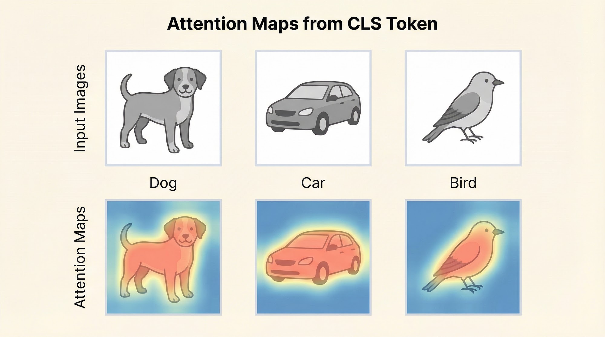
One of the most fascinating aspects of Vision Transformers is the ability to visualize attention maps — which show where the model "looks" for each patch. When you visualize the attention from the [CLS] token to all image patches, you find that the model learns to focus on semantically meaningful regions. For an image of a dog, the attention concentrates on the dog's face and body. For an image of a car, it concentrates on the car itself, ignoring the background.

This is truly amazing. Without any explicit instruction about what objects are or where they are, the self-attention mechanism discovers object-level structure purely from the classification objective.

Attention maps reveal that ViT learns to focus on semantically meaningful regions.

Summary and What Comes Next

Let us take a step back and look at the journey we have taken.

We started with the convolution — a simple operation that slides a learnable filter across an image to detect local patterns. By stacking convolutions, we built Convolutional Neural Networks that progressively extract higher-level features: edges, textures, parts, objects. For nearly a decade, CNNs were the undisputed champions of computer vision.

Then we encountered a fundamental limitation: CNNs process images locally, and capturing long-range relationships requires stacking many layers. This led to the Vision Transformer, which takes a radically different approach: split the image into patches, treat them as tokens, and let every patch attend to every other patch through self-attention.

Both paradigms have their strengths. CNNs excel when data is limited, thanks to their built-in inductive biases. Vision Transformers excel when data is abundant, thanks to their flexibility and scalability. And increasingly, the best models combine both approaches.

Today, vision encoders are the backbone of multimodal AI systems like CLIP (which aligns images and text in a shared embedding space), SigLIP, and vision-language models that power applications from medical imaging to autonomous driving. Understanding how they work — from the humble convolution to the global self-attention mechanism — is essential for anyone working in modern AI.

References:

LeCun, Y. et al. (1998). "Gradient-based learning applied to document recognition." Proceedings of the IEEE.
Krizhevsky, A. et al. (2012). "ImageNet classification with deep convolutional neural networks." NeurIPS.
He, K. et al. (2016). "Deep residual learning for image recognition." CVPR.
Vaswani, A. et al. (2017). "Attention is all you need." NeurIPS.
Dosovitskiy, A. et al. (2020). "An image is worth 16x16 words: Transformers for image recognition at scale." ICLR 2021.
Touvron, H. et al. (2021). "Training data-efficient image transformers & distillation through attention." ICML.

That's it!