Basics of Reinforcement Learning: Teaching Machines to Learn from Experience

From the agent-environment loop to Bellman equations, rewards, and your first OpenAI Gymnasium agent -- all from first principles.

---

Let us start with a simple example. Imagine a child learning to ride a bicycle. Nobody hands the child a dataset of "correct bicycle movements." Nobody clusters the child's experiences into groups. Instead, the child gets on the bicycle, wobbles, falls, gets a scraped knee (a negative reward), tries again, adjusts the handlebars slightly differently, and eventually -- after dozens of attempts -- learns to balance and pedal smoothly.

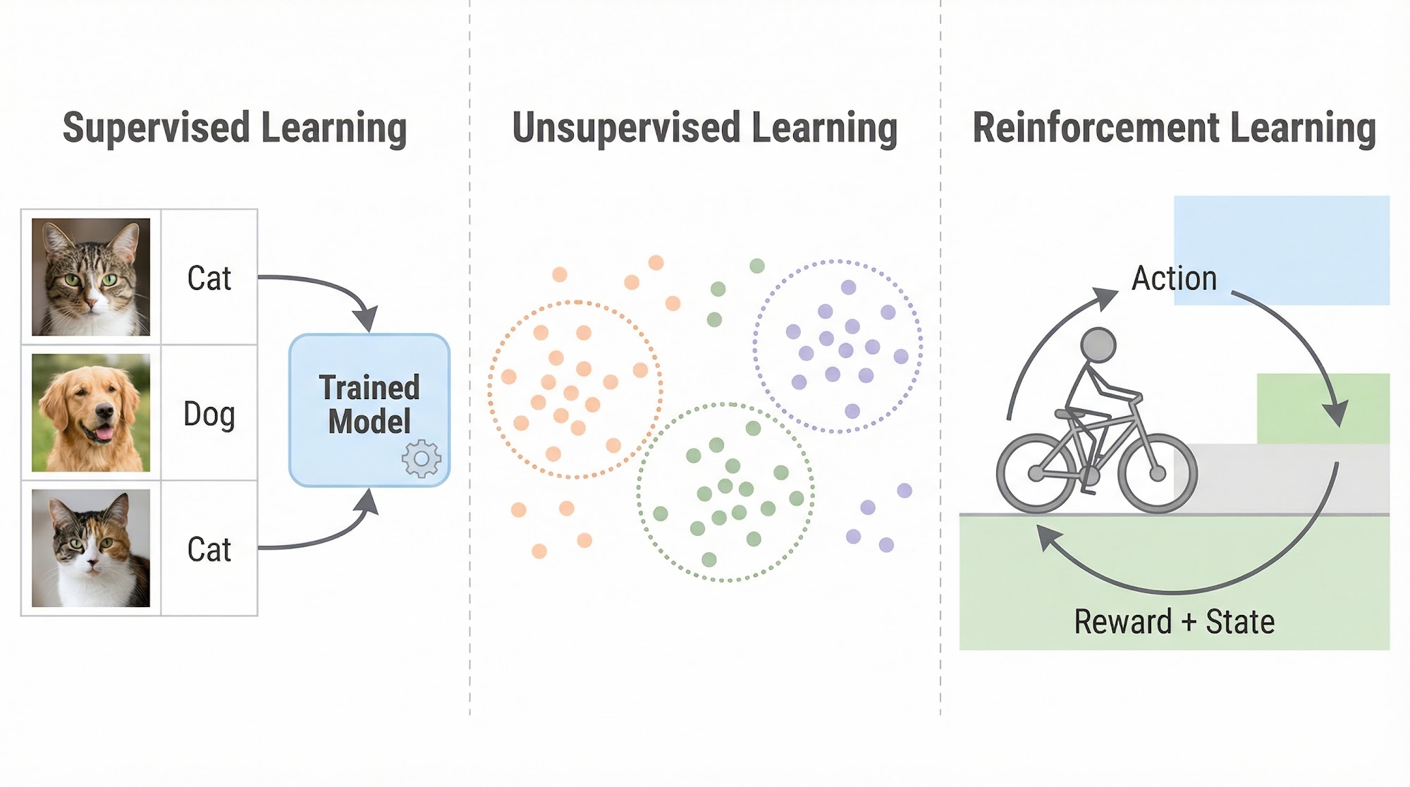
This is fundamentally different from the two forms of machine learning you may already know. In supervised learning, we hand the model a labeled dataset -- here are 1,000 images of cats, here are 1,000 images of dogs, now learn to tell them apart. In unsupervised learning, we hand the model unlabeled data and ask it to find hidden patterns or clusters on its own.

But what if the model has no dataset at all? What if, instead of learning from pre-collected data, the model learns by interacting with the world -- taking actions, observing consequences, and adjusting its behavior to maximize some notion of reward?

This brings us to the field of reinforcement learning.

The three paradigms of machine learning compared side by side.

The Reinforcement Learning Problem

To appreciate what makes reinforcement learning special, let us look at a few real-world examples.

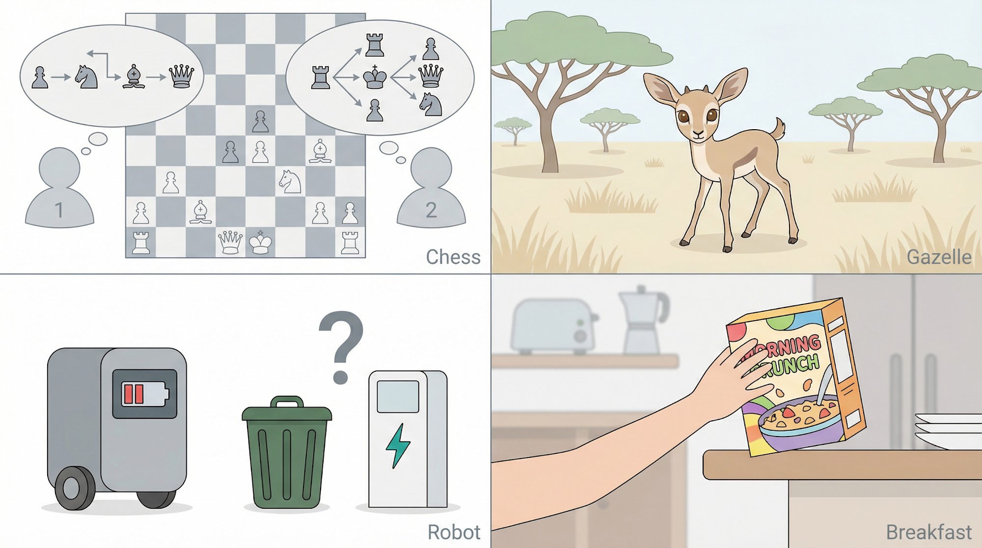
(1) A master chess player makes a move. The choice is based on two things: planning by anticipating replies and counter-replies, and intuitive judgment about the desirability of positions. The player does not have a labeled dataset of "correct moves" -- they learn through thousands of games.

(2) A gazelle calf learning to run. The calf struggles to stand 2-3 minutes after birth. However, after just 30 minutes, it is running at 36 km/hr. It learns entirely through trial and error, with the environment providing feedback at every step.

(3) A mobile robot deciding whether to search for trash or recharge. The robot must weigh its current battery level against the potential reward of finding more trash. This decision involves balancing immediate and long-term rewards.

(4) Phil preparing his breakfast. Walking to the cupboard, opening it, selecting a cereal box, reaching for a plate and spoon -- each step is guided by goals in service of other goals, with the ultimate goal of obtaining nourishment.

What is common in all these examples?

In every case, the agent uses its experience to improve its performance over time by interacting with the environment. There is no teacher providing the right answer. There is no pre-collected dataset. The agent learns from the consequences of its own actions.

Four real-world examples of agents learning from interaction.

Of all the forms of machine learning, reinforcement learning is the closest to the kind of learning that humans and other animals do. Many of its core algorithms were originally inspired by biological learning systems.

Now let us formalize this. The goal of a reinforcement learning agent can be written mathematically as:

$$\max_{\pi} \; \mathbb{E}\left[\sum_{t=0}^{T} r_t\right]$$

Here, $\pi$ is the agent's policy (the strategy it follows), $r_t$ is the reward at time step $t$, and $T$ is the final time step. The agent wants to find the policy that maximizes the total expected reward over the entire episode.

Let us plug in some simple numbers to see how this works. Suppose a robot collects cans over 3 time steps and receives rewards $r_0 = 1$, $r_1 = 0$, $r_2 = 1$. Then the total reward is:

$$\sum_{t=0}^{2} r_t = 1 + 0 + 1 = 2$$

The agent's goal is to find a policy that makes this sum as large as possible. This is exactly what we want.

The Four Elements of Reinforcement Learning

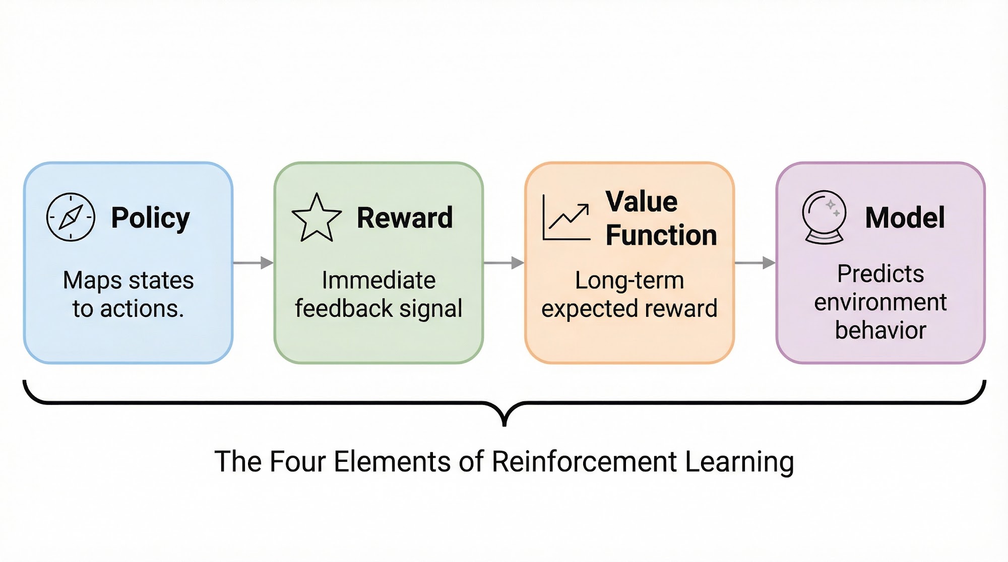
Every reinforcement learning system has four key elements. Let us understand each one.

(1) Policy. Informally, the policy defines the agent's way of behaving at a given time. Formally, the policy is a mapping from perceived states of the environment to actions taken when in those states. If you are playing chess and your policy says "when the opponent's queen is unprotected, capture it," that is a specific mapping from a state (unprotected queen) to an action (capture).

(2) Reward Signal. The reward signal defines the goal of the reinforcement learning problem. At each time step, the environment sends the agent a single number: the reward. The sole objective of the agent is to maximize the total reward received over time. The reward is analogous to pleasure or pain in a biological system -- if you touch a boiling vessel, your body gives you a very strong negative reward signal.

(3) Value Function. While the reward signal indicates what is good in an immediate sense, the value function specifies what is good in the long run. The value of a state is the total amount of reward the agent can expect to accumulate over the future, starting from that state.

Consider a cricket tournament with 14 matches. A new player does not perform well in the first two matches -- the immediate reward is low. But the captain has faith that the player will improve in later matches. Even though the reward signal is currently low, the value is high because the long-term desirability of keeping this player is high.

"In the field of reinforcement learning, the central role of value estimation is the most important thing that researchers learned from 1960 to 1990."

(4) Model of the Environment. The model mimics the behavior of the environment, allowing the agent to predict what will happen next. There are model-based methods (which learn or use a model) and model-free methods (which learn directly from experience without a model).

The four foundational elements of every RL system.

Let us look at a practical example to see these elements in action. Consider the game of Tic-Tac-Toe.

Our goal is to build a player that can find flaws in the opponent's play and maximize the chances of winning.

State: The configuration of X's and O's on the 3x3 board.

Policy: A rule which tells the player what move to make for every state of the game.

Value Function: For every state, we assign a number which gives our latest estimate of the probability of winning from that state.

Have a look at the value function table below.

Value function assigns winning probability to each game state.

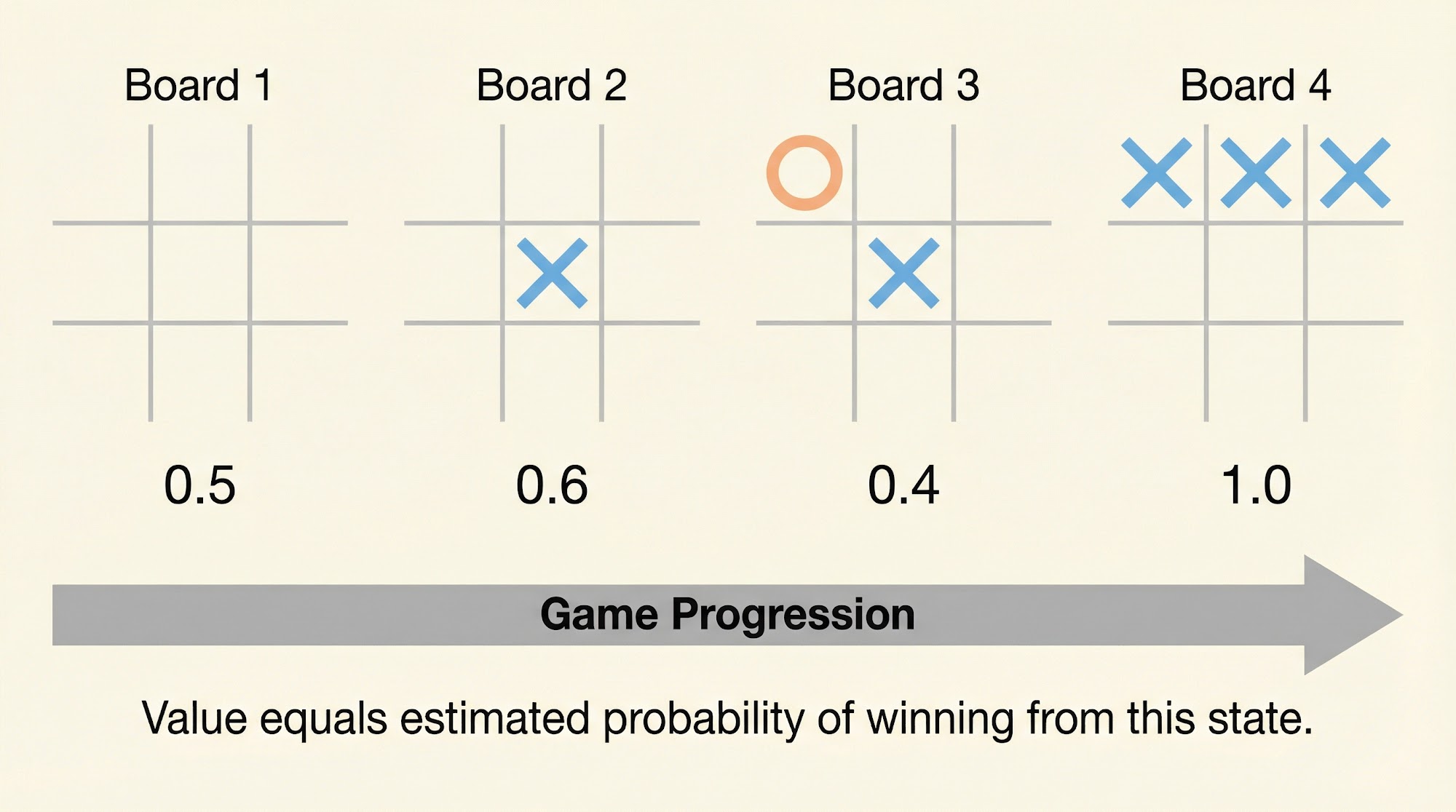
The value function estimates change as the agent plays more games. Now, suppose we are playing "X" and we face a board with several possible next moves. We look at all possible next states and select the one with the highest estimated probability of winning. This is called exploitation -- selecting the state with the greatest value.

But sometimes, we select randomly from the available states so that we can experience states we might otherwise never see. This is called exploration. The balance between exploitation and exploration is one of the central challenges in reinforcement learning.

After each move, we adjust the value of the earlier state to be closer to the value of the next state. This process is called backing up, and it is how the agent gradually learns to make better decisions.

The Agent-Environment Interface

The most common framework for representing reinforcement learning problems is the agent-environment interface.

The agent-environment interface loop: at each step the agent observes state, takes action, receives reward.

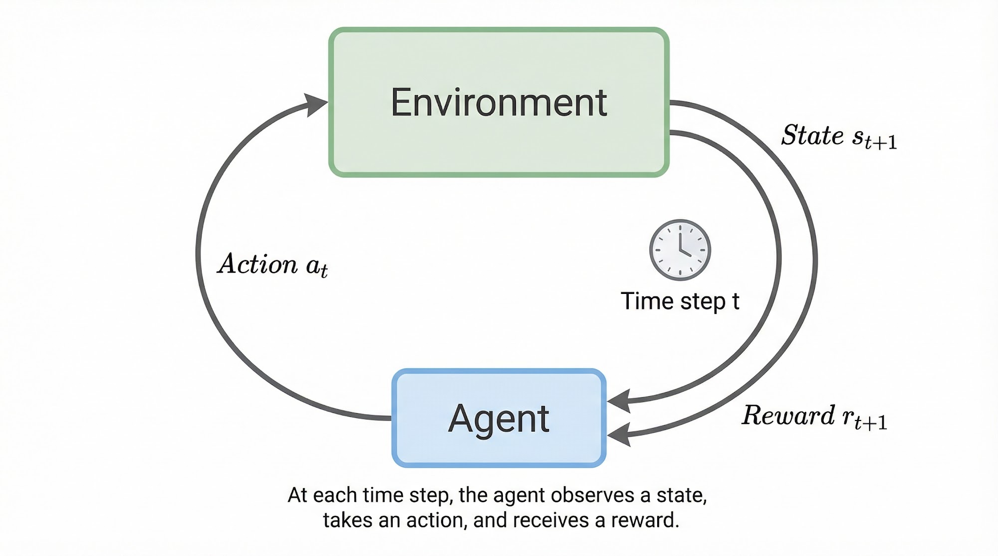
At each time step $t$, the agent receives information about the state of the environment $s_t$. Based on this state, the agent performs an action $a_t$. One time step later, the agent receives a reward $r_{t+1}$ and observes a new state $s_{t+1}$.

Formally, a Markov Decision Process is defined by the tuple:

$$\text{MDP} = (S, A, P, R, \gamma)$$

Here, $S$ is the set of all states, $A$ is the set of all actions, $P$ is the transition probability function, $R$ is the reward function, and $\gamma$ is the discount factor.

Let us plug in some simple numbers. Suppose we have a tiny environment with $S = \{s_1, s_2\}$ (two states), $A = \{a_1, a_2\}$ (two actions), and $\gamma = 0.9$. If the agent is in state $s_1$ and takes action $a_1$, it might transition to state $s_2$ with probability $P(s_2 | s_1, a_1) = 0.8$ and stay in $s_1$ with probability $P(s_1 | s_1, a_1) = 0.2$. The reward might be $R(s_1, a_1) = 5$. This tells us that taking action $a_1$ in state $s_1$ gives an immediate reward of 5 and most likely moves us to state $s_2$.

Let us look at two practical examples to make this concrete.

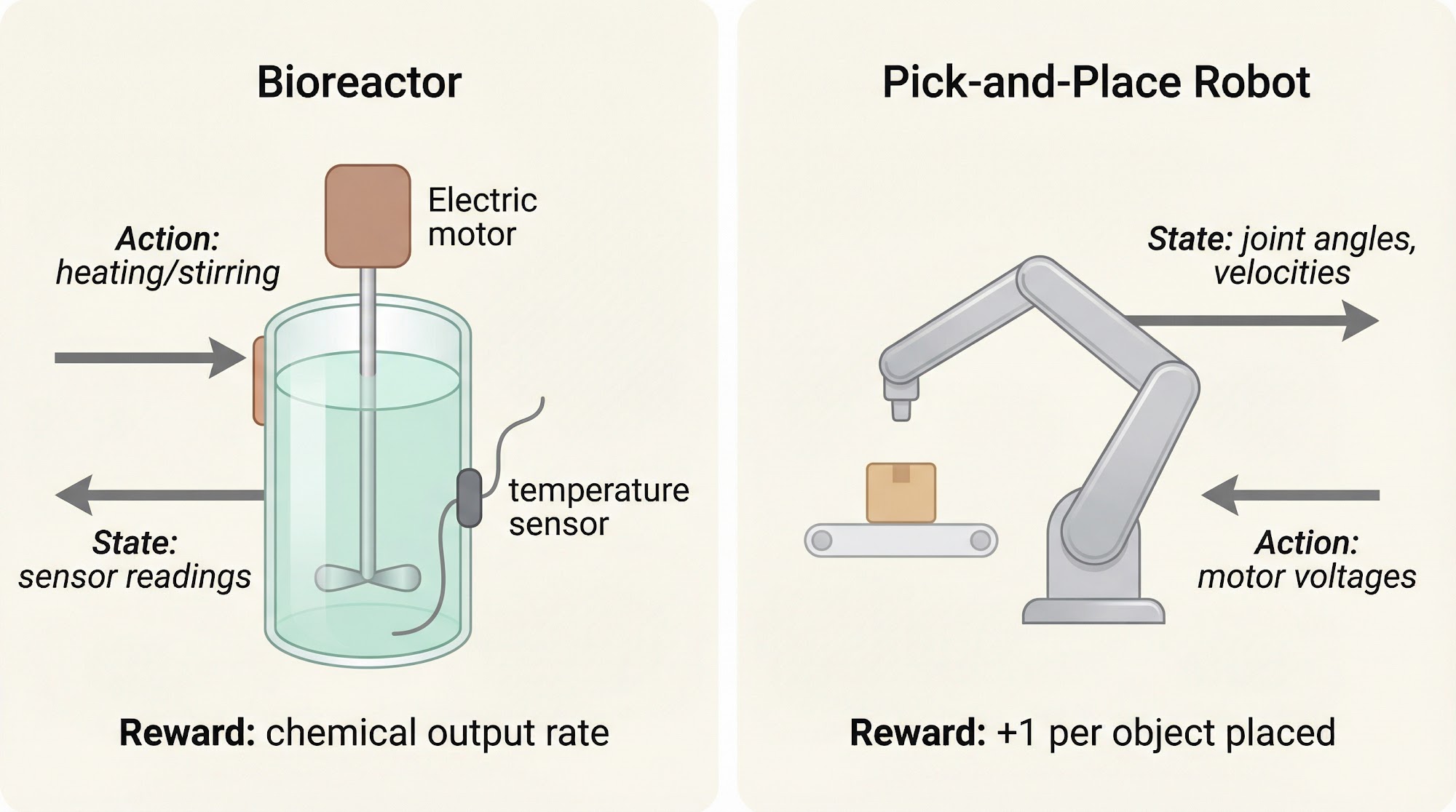
Example 1: Bioreactor. The states are sensor readings and thermocouple readings. The actions are activating the heating element (to reach a target temperature) and activating motors (to reach a target stirring rate). The rewards are the moment-to-moment measures of the rate at which useful chemicals are produced.

Example 2: Pick-and-Place Robot. The states are readings of joint angles and velocities. The actions are voltages applied to motors at each joint. The reward is +1 for each object successfully picked and placed, and -0.02 for jerky motion.

Two real-world RL examples: a bioreactor controlling chemical output and a pick-and-place robot learning motor control.

Rewards and Returns

The use of a reward signal to formalize the idea of a goal is one of the most distinctive features of reinforcement learning. Let us look at some examples.

(1) Game of Chess: Reward is +1 for winning, -1 for losing, 0 for a draw.

(2) Robot escaping a maze: Reward is -1 for every time step that passes before the robot escapes.

(3) Robot collecting empty soda cans: Reward is +1 for each can collected, 0 otherwise.

We should be careful in designing rewards. Rewards should be given for achieving the actual goal, not for sub-goals. For example, giving a chess agent a reward for capturing the opponent's queen might teach it to prioritize queen-capture over winning the game.

Now let us understand returns. The goal of the agent is to maximize the cumulative reward it receives in the long run. We call this the expected return:

$$G_t = r_t + r_{t+1} + r_{t+2} + \cdots + r_T$$

Here, $T$ denotes the final time step. This formulation works for episodic tasks -- tasks with a natural ending, like a game of chess or a trip through a maze.

Let us plug in some simple numbers. Suppose a robot collects cans over 4 time steps with rewards $r_0 = 1$, $r_1 = 0$, $r_2 = 1$, $r_3 = 1$. The return is:

$$G_0 = 1 + 0 + 1 + 1 = 3$$

This tells us the total reward collected from time step 0 onward is 3. The agent wants to find a policy that makes this as large as possible.

But what about tasks that go on continuously, like a rover on a Mars expedition? These are called continuing tasks, and the return could become infinite. We naturally come to the concept of discounting.

Let us understand discounting with an analogy. Rs. 100 are more valuable now compared to five years later due to inflation. Similarly, immediate rewards are more valuable compared to rewards received later. We account for this by saying that every reward is $\gamma$ times less valuable than the reward before, where $\gamma$ is the discount factor and $0 \leq \gamma < 1$.

The discounted return is:

$$G_t = r_t + \gamma \, r_{t+1} + \gamma^2 \, r_{t+2} + \gamma^3 \, r_{t+3} + \cdots = \sum_{k=0}^{\infty} \gamma^k \, r_{t+k}$$

If $\gamma = 0$, the agent only cares about immediate rewards. As $\gamma$ approaches 1, the agent considers future rewards more strongly.

Let us plug in some simple numbers. Suppose our rewards are $r_t = 1$, $r_{t+1} = 2$, $r_{t+2} = 3$, and $\gamma = 0.9$:

$$G_t = 1 + 0.9 \times 2 + 0.81 \times 3 = 1 + 1.8 + 2.43 = 5.23$$

This tells us that our total discounted return from time step $t$ is 5.23. Notice how the later rewards contribute less due to discounting -- this is exactly what we want.

Let us look at a great example to illustrate the difference between episodic and continuing formulations. Consider the classic Cart-Pole problem.

The cart-pole environment with episodic vs continuing reward formulations.

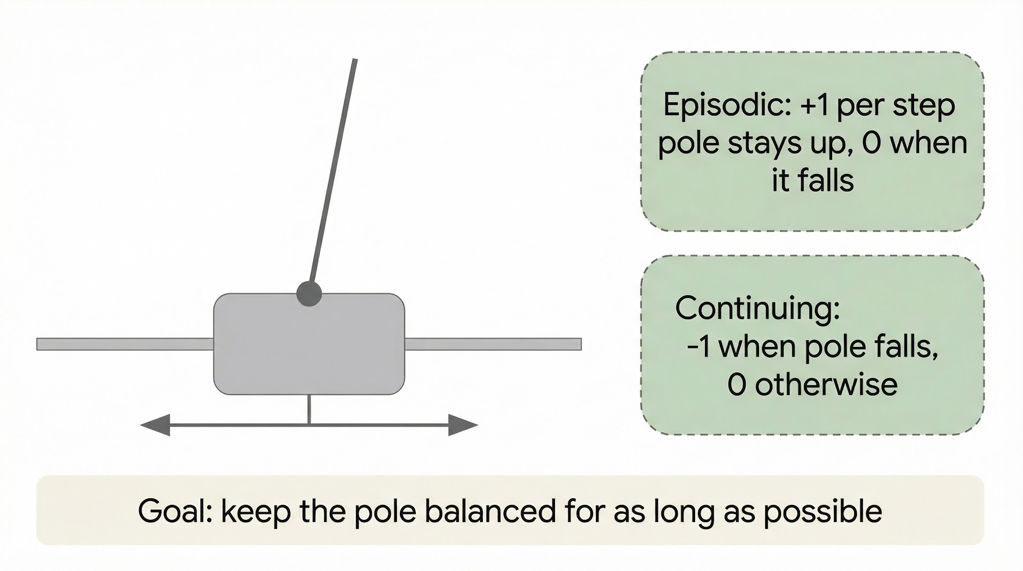
Option 1: Episodic formulation. Reward = +1 for every time step the pole stays upright, 0 when it falls. The return is maximized only if the pole stays up for the maximum number of time steps. This is exactly what we want.

Option 2: Continuing formulation. Reward = -1 when the pole falls, 0 otherwise. The return is maximized if failure occurs as late as possible. This is also what we want.

Both formulations lead to the same desired behavior, but through different reward structures.

The Markov Property

We know that the agent makes a decision after receiving a state signal from the environment. Let us look at state signals that have a very special property.

Conversations: When we are speaking with someone, the entire history of our past conversation is known to us -- it is all stored in the current state of the dialogue.

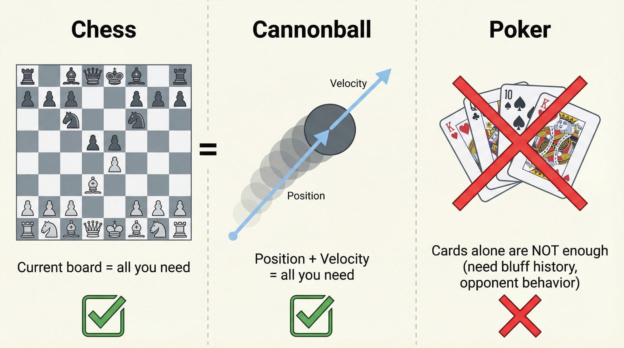
Chess: The current configuration of chess pieces on the board contains all the information needed -- you do not need to know the entire history of how the pieces got there.

Cannonball: The current position and velocity of a cannonball are all that is needed to predict its future trajectory. Past positions do not add any additional information.

What is common in all these examples?

In each case, the current state retains all the relevant information from the past. A state signal that succeeds in maintaining all relevant information is said to have the Markov property.

Chess and cannonball satisfy the Markov property; poker does not.

Formally, a state has the Markov property if:

$$P(s_{t+1} \mid s_t, a_t) = P(s_{t+1} \mid s_0, a_0, s_1, a_1, \ldots, s_t, a_t)$$

This says that the probability of transitioning to the next state depends only on the current state and action, not on the entire history.

Let us plug in some simple numbers. Suppose we have three states: $s_1, s_2, s_3$. If the system is Markov, then $P(s_3 | s_2, a) = 0.7$ regardless of whether we visited $s_1$ before $s_2$ or arrived at $s_2$ directly. The history does not matter -- only the current state does. This makes computation enormously simpler, because we do not need to track the entire past.

An interesting counter-example is the game of Draw Poker. For the state to satisfy the Markov property, the player would need to know: their own cards, all bets made, the number of cards drawn by opponents, and even the bluffing history of opponents. Nobody remembers this much information while playing poker. Unless you are James Bond :)

Hence, the state representations people use for poker decisions are typically non-Markov.

Markov Decision Processes

A reinforcement learning task that satisfies the Markov property is called a Markov Decision Process (MDP). Let us look at a practical example.

Consider a recycling robot. At each time step, the robot decides between three actions: actively search for a can, remain stationary and wait for someone to bring a can, or go back to home base and recharge the battery.

The robot has two possible states: High (battery level high) and Low (battery level low).

The rewards are as follows: $r_{\text{search}}$ is the expected number of cans collected while searching, $r_{\text{wait}}$ is the expected number of cans received while waiting, and -3 is the penalty if the battery dies and the robot must be rescued.

A period of searching that starts with high energy leaves the level high with probability $\alpha$ and reduces it to low with probability $1 - \alpha$. A period of searching starting with low energy leaves the level low with probability $\beta$ and depletes the battery with probability $1 - \beta$.

State transition diagram for the recycling robot MDP.

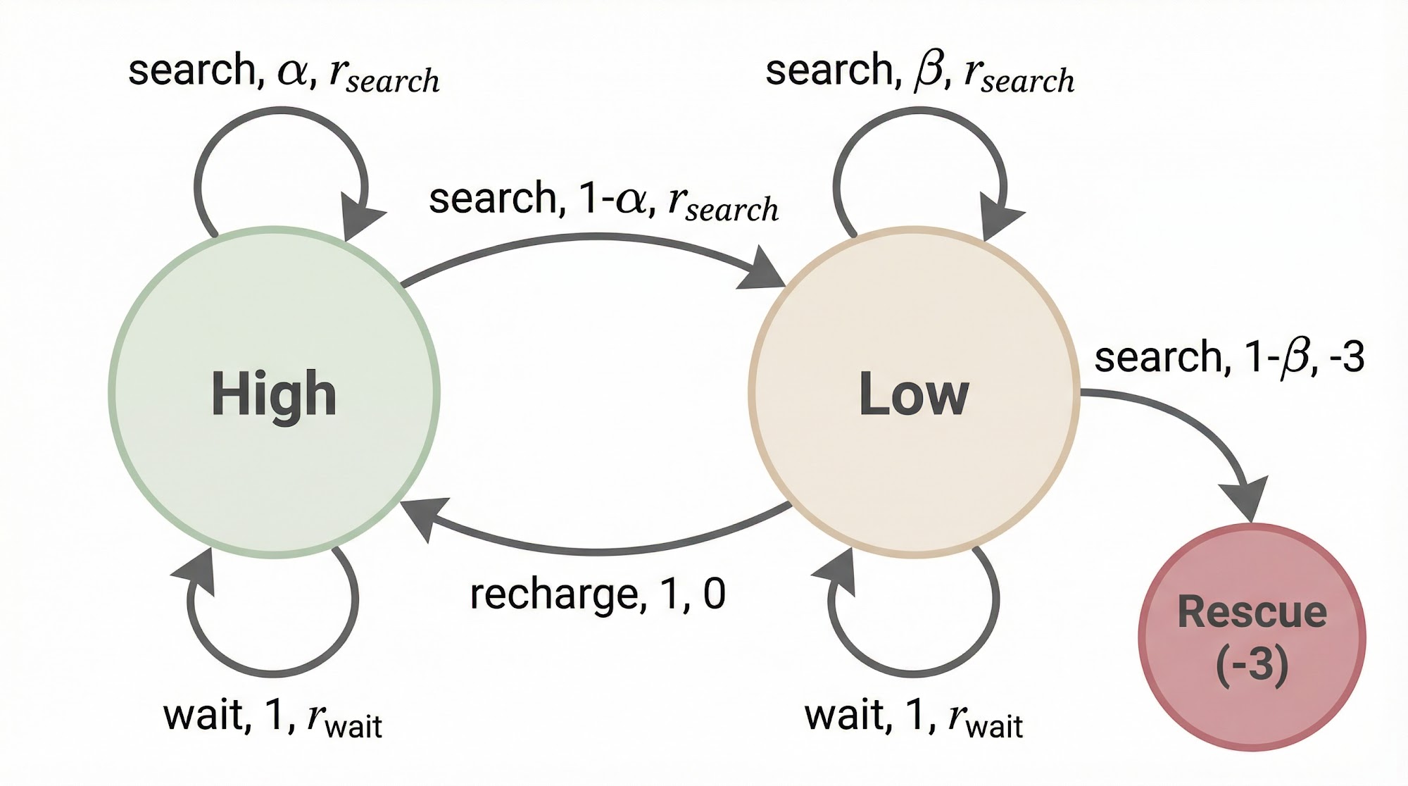
Let us plug in some simple numbers to make this concrete. Suppose $\alpha = 0.7$, $\beta = 0.4$, $r_{\text{search}} = 2$, $r_{\text{wait}} = 1$. If the robot is in the High state and decides to search, there is a 70% chance it stays in High and a 30% chance it drops to Low, collecting an expected reward of 2 cans either way. If it waits, it stays High with certainty but only collects 1 can. If the robot is in the Low state and searches, there is a 40% chance it stays Low and a 60% chance the battery dies (penalty of -3). This is exactly why the recharge action exists -- sometimes it is better to sacrifice short-term reward for long-term survival.

OpenAI Gymnasium -- Practical Implementation

Enough theory, let us look at some practical implementation now. Reinforcement learning has always been thought of as a very theoretical field, but it is surprisingly simple to get started practically.

The Python library called Gym was developed by OpenAI in 2017. In 2021, the team moved development to Gymnasium. The main goal of Gymnasium is to provide a rich collection of RL environments with a unified interface.

Gymnasium provides the following:

• Set of actions allowed in the environment (discrete or continuous)
• Shape and boundaries of the observations
• A step method to execute an action and return the current observation, reward, and episode status
• A reset method to return the environment to its initial state

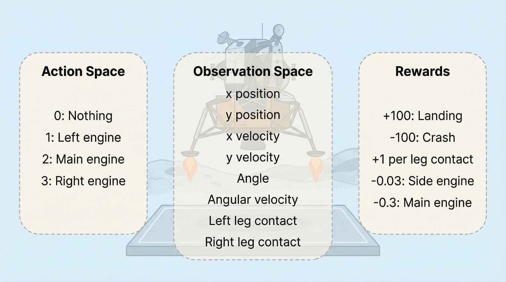
Let us look at the Lunar Lander environment.

The Lunar Lander environment from OpenAI Gymnasium with action space, observation space, and reward structure.

Now let us write our first code. First, install the dependency:

pip install gymnasium[box2d]

That's all! Now let us create the environment and explore it:

import gymnasium as gym

# Create the environment
env = gym.make("LunarLander-v3")

# Sample an action from the action space
sample_action = env.action_space.sample()
print("Sample action from action space:", sample_action)

# Sample an observation from the observation space
sample_observation = env.observation_space.sample()
print("Sample observation from observation space:", sample_observation)

# Check the space definitions
print("Action space:", env.action_space)
print("Observation space:", env.observation_space)

env.close()

This code will give you a sample action from the action space and a sample observation from the observation space. There are three key functions here:

• gym.make() creates the environment
• env.action_space.sample() samples a random action
• env.observation_space.sample() samples a random observation

You might be thinking: but I never defined the action space or the observation space. They are defined inside the environment for you.

Now let us actually control our lunar lander. The following code runs the lander with random actions -- no policy at all:

import gymnasium as gym

# Create the environment with visual rendering
env = gym.make("LunarLander-v3", render_mode="human")

env.reset()

for step in range(200):
    env.render()
    env.step(env.action_space.sample())

env.close()

Let us understand this code in detail. The gym.make() function creates our environment. The env.reset() function resets the episode and collects the first observation -- this is a mandatory step. Then, for 200 steps, we render the environment and take a random action using env.action_space.sample().

The env.step() function takes an action as input and returns five things:

1. Observation -- the agent's view of the environment after the action
2. Reward -- the reward received from this action
3. Terminated -- whether a terminal state has been reached
4. Truncated -- whether the episode ended prematurely (due to time limits or going out of bounds)
5. Info -- a dictionary of diagnostic information for debugging

Random agent vs trained agent: the difference a policy makes.

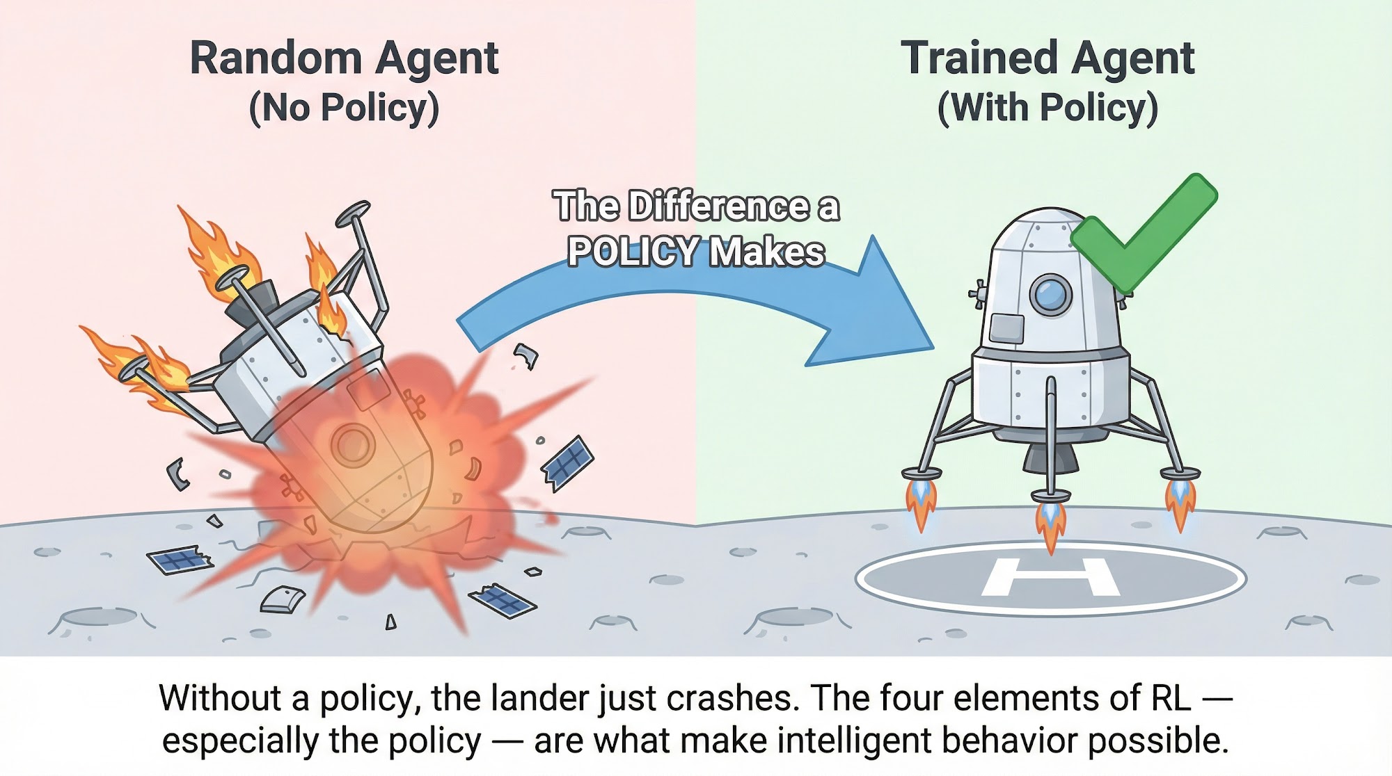
Once you run this code, you will see a PyGame window with the lunar lander moving toward the surface. You might be wondering: well, this is not very good. Our lunar lander just falls off -- it is not oriented properly and crashes.

If only it was this easy to run reinforcement learning problems :)

To understand why we are not doing well, go back and check the four elements of reinforcement learning. We have missed a major element.

Yes -- the policy.

We are taking random actions, which means we have no intelligent strategy for choosing which thruster to fire. The missing piece is a policy that tells the agent which action to take in each state to maximize cumulative reward.

Wrapping Up

Let us recap what we have covered. We started with the fundamental question: how can a machine learn from interaction rather than from data? We saw that reinforcement learning is defined by the interplay of four elements -- the policy, the reward signal, the value function, and the model of the environment. We formalized the problem using Markov Decision Processes and the agent-environment interface. We learned about rewards, returns, discounting, and the Markov property. And we got our hands dirty with OpenAI Gymnasium, seeing firsthand why a random agent is not enough.

The natural next step is to learn how to build an actual policy. How do we teach the agent which actions are good in which states? This is where value functions, the Bellman equation, and algorithms like Q-learning come in.

Play around with Gymnasium and try various environments. The code is available on GitHub: https://github.com/RajatDandekar/Hands-on-RL-Bootcamp-Vizuara

That's it for now. See you next time!

---

References:

1. Sutton, R.S. and Barto, A.G. (2018). Reinforcement Learning: An Introduction. 2nd Edition. MIT Press.
2. OpenAI Gymnasium Documentation: https://gymnasium.farama.org/
3. Bellman, R. (1957). Dynamic Programming. Princeton University Press.