Denoising Diffusion Probabilistic Models (DDPM) — From Noise to Crystal-Clear Images

A step-by-step guide to understanding how DDPMs learn to generate images by mastering the art of denoising

Let us start with a simple thought experiment. Imagine you have a beautiful photograph of a cat. Now, suppose someone starts corrupting this image — at each step, they add a tiny bit of random static noise to every pixel. After one step, the image looks almost the same. After ten steps, it looks slightly grainy. After a hundred steps, the cat is barely recognizable. And after a thousand steps, all you see is pure, meaningless static — like the snow on an old television screen.

Now here is the interesting question: Can you learn to reverse this process? Can you take that pile of random noise and, step by step, reconstruct the original cat photograph?

This is exactly what Denoising Diffusion Probabilistic Models (DDPMs) do. The idea was formalized by Ho, Jain, and Abbeel in their landmark 2020 paper, and it has since become one of the most influential frameworks in generative AI.

The core idea is beautifully simple:

Forward process: Systematically destroy an image by adding noise over many small steps until nothing remains but pure Gaussian noise.
Reverse process: Train a neural network to undo each step of noise addition, learning to progressively reconstruct the original image from noise.

If the network learns to reverse each tiny step of corruption, then we can start from pure random noise and generate entirely new images that look like they came from the training data.

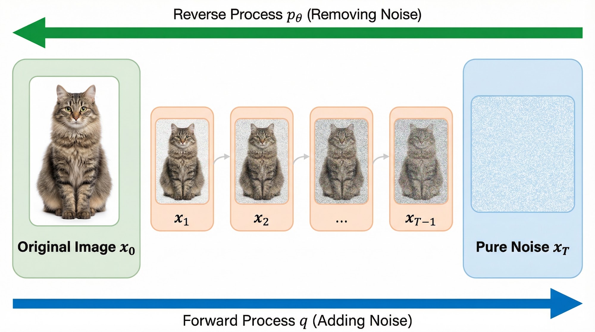
The forward process destroys structure; the reverse process reconstructs it.

Let us now understand each of these processes in detail.

The Forward Process — Destroying Images Systematically

Let us begin by understanding how we systematically destroy an image. The forward process takes a clean image and gradually adds Gaussian noise to it over T time steps.

At each step t, we take the image from the previous step and add a small amount of noise. The mathematical representation for a single step is:

q(\mathbf{x}_t | \mathbf{x}_{t-1}) = \mathcal{N}\left(\mathbf{x}_t; \sqrt{1 - \beta_t}\, \mathbf{x}_{t-1},\; \beta_t \mathbf{I}\right)

What does this mean? For each pixel, we sample from a Gaussian distribution where:

The mean is the previous pixel value scaled down by a factor of $\sqrt{1 - \beta_t}$
The variance is $\beta_t$

The parameter $\beta_t$ is called the noise schedule. It controls how much noise is added at each step. Typically, $\beta_t$ starts small (e.g., $\beta_1 = 0.0001$ ) and increases linearly to a larger value (e.g., $\beta_T = 0.02$ ).

Let us plug in some simple numbers to see how this works. Suppose we have a single pixel with value $x_{t-1} = 0.8$ , and at this time step $\beta_t = 0.01$ .

The mean of the Gaussian is $\sqrt{1 - 0.01} \times 0.8 = \sqrt{0.99} \times 0.8 = 0.995 \times 0.8 = 0.796$ .

The variance is $0.01$ , so the standard deviation is $\sqrt{0.01} = 0.1$ .

So the new pixel value is sampled from $\mathcal{N}(0.796, 0.1^2)$ . Notice how the mean has shrunk slightly (from 0.8 to 0.796) and we have added a small amount of random noise. After many such steps, the pixel value will drift towards zero and the noise will dominate. This is exactly what we want.

Forward diffusion progressively transforms a clean digit into pure Gaussian noise.

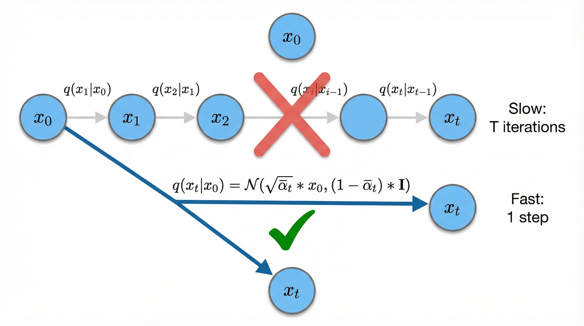
Now, here is a clever mathematical trick. For convenience, let us define $\alpha_t = 1 - \beta_t$ and $\bar{\alpha}_t = \prod_{s=1}^{t} \alpha_s$ . Using these definitions, we can derive a closed-form expression that lets us jump directly from the original image $\mathbf{x}_0$ to any noisy version $\mathbf{x}_t$ in a single step:

q(\mathbf{x}_t | \mathbf{x}_0) = \mathcal{N}\left(\mathbf{x}_t;\; \sqrt{\bar{\alpha}_t}\, \mathbf{x}_0,\; (1 - \bar{\alpha}_t)\, \mathbf{I}\right)

This means we can write:

\mathbf{x}_t = \sqrt{\bar{\alpha}_t}\, \mathbf{x}_0 + \sqrt{1 - \bar{\alpha}_t}\, \boldsymbol{\epsilon}, \quad \boldsymbol{\epsilon} \sim \mathcal{N}(\mathbf{0}, \mathbf{I})

This is extremely important for training, because we do not have to iteratively add noise T times — we can jump to any noise level in one step.

Let us plug in some numbers. Suppose $\bar{\alpha}_t = 0.5$ (which means about half the original signal is preserved) and our pixel value is $x_0 = 0.8$ . If we sample $\epsilon = 0.3$ from a standard Gaussian:

$x_t = \sqrt{0.5} \times 0.8 + \sqrt{1 - 0.5} \times 0.3 = 0.707 \times 0.8 + 0.707 \times 0.3 = 0.566 + 0.212 = 0.778$

At $\bar{\alpha}_t = 0.5$ , about 70.7% of the original signal remains and 70.7% of the noise is mixed in. As $\bar{\alpha}_t$ decreases towards zero (at later time steps), the noise completely takes over. This makes sense because the forward process should eventually destroy all structure in the image.

The closed-form formula lets us skip directly to any noise level in one step.

The Reverse Process — Learning to Denoise

Now let us come to the main character in our story: the reverse process.

Our goal is to start from pure noise $\mathbf{x}_T \sim \mathcal{N}(\mathbf{0}, \mathbf{I})$ and progressively remove noise until we get a clean image. To do this, we need to learn the reverse transition $p(\mathbf{x}_{t-1} | \mathbf{x}_t)$ .

But here is the problem: computing $q(\mathbf{x}_{t-1} | \mathbf{x}_t)$ directly is intractable. It would require integrating over all possible original images, which is impossible.

However, there is a beautiful result. If we also condition on the original image $\mathbf{x}_0$ , the posterior becomes tractable. It turns out that $q(\mathbf{x}_{t-1} | \mathbf{x}_t, \mathbf{x}_0)$ is a Gaussian distribution with a known mean and variance:

q(\mathbf{x}_{t-1} | \mathbf{x}_t, \mathbf{x}_0) = \mathcal{N}\left(\mathbf{x}_{t-1};\; \tilde{\boldsymbol{\mu}}_t(\mathbf{x}_t, \mathbf{x}_0),\; \tilde{\beta}_t \mathbf{I}\right)

where the mean is:

\tilde{\boldsymbol{\mu}}_t(\mathbf{x}_t, \mathbf{x}_0) = \frac{\sqrt{\bar{\alpha}_{t-1}}\, \beta_t}{1 - \bar{\alpha}_t}\, \mathbf{x}_0 + \frac{\sqrt{\alpha_t}\,(1 - \bar{\alpha}_{t-1})}{1 - \bar{\alpha}_t}\, \mathbf{x}_t

and the variance is:

\tilde{\beta}_t = \frac{(1 - \bar{\alpha}_{t-1})}{(1 - \bar{\alpha}_t)} \cdot \beta_t

Let us plug in some concrete numbers to understand this. Suppose at time step $t = 500$ (out of $T = 1000$ ), we have $\alpha_t = 0.99$ , $\bar{\alpha}_t = 0.5$ , $\bar{\alpha}_{t-1} = 0.505$ , $\beta_t = 0.01$ . If $x_0 = 0.8$ (original pixel) and $x_t = 0.6$ (current noisy pixel):

The coefficient of $x_0$ is $\frac{\sqrt{0.505} \times 0.01}{1 - 0.5} = \frac{0.711 \times 0.01}{0.5} = \frac{0.00711}{0.5} = 0.0142$

The coefficient of $x_t$ is $\frac{\sqrt{0.99} \times (1 - 0.505)}{1 - 0.5} = \frac{0.995 \times 0.495}{0.5} = \frac{0.4925}{0.5} = 0.985$

So $\tilde{\mu}_t = 0.0142 \times 0.8 + 0.985 \times 0.6 = 0.0114 + 0.591 = 0.602$

This tells us that the true reverse step mostly relies on the current noisy image $x_t$ (with coefficient 0.985) and only slightly uses the original image $x_0$ (with coefficient 0.0142). This makes intuitive sense — at intermediate noise levels, the noisy image still contains a lot of useful information.

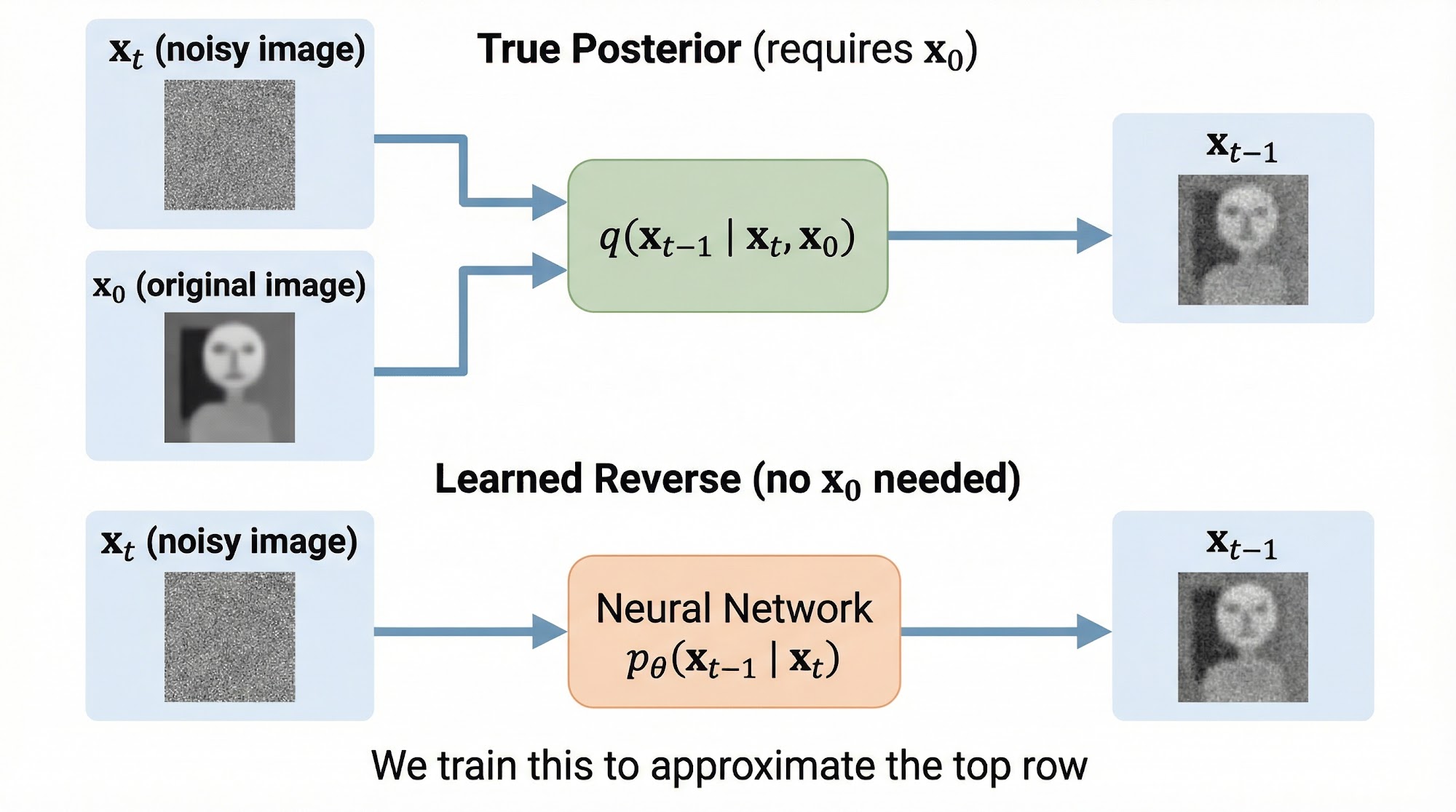
The neural network learns to approximate the true posterior without the original image.

But wait — during generation, we do not have access to $\mathbf{x}_0$ ! That is the whole point: we are trying to generate new images, so we cannot condition on the original.

This is where the neural network comes in. We train a model $p_\theta$ to approximate the reverse process:

p_\theta(\mathbf{x}_{t-1} | \mathbf{x}_t) = \mathcal{N}\left(\mathbf{x}_{t-1};\; \boldsymbol{\mu}_\theta(\mathbf{x}_t, t),\; \sigma_t^2 \mathbf{I}\right)

The model outputs a predicted mean $\boldsymbol{\mu}_\theta(\mathbf{x}_t, t)$ , and we fix the variance to be either $\beta_t$ or $\tilde{\beta}_t$ (both work well in practice). The model takes as input the noisy image $\mathbf{x}_t$ and the timestep $t$ , and it learns to predict what the slightly less noisy image should look like.

The DDPM Loss — Predicting the Noise

Now the question is: How do we train this neural network?

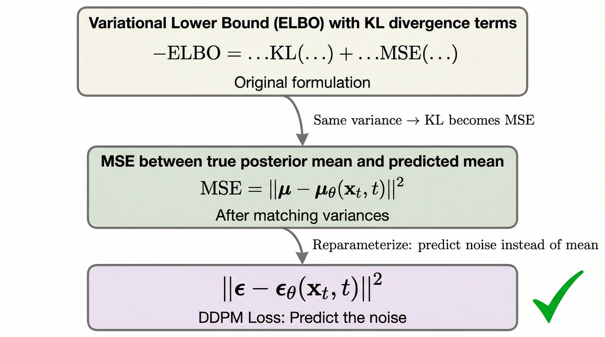
We start from the variational lower bound, just as we did for VAEs. The evidence lower bound (ELBO) for diffusion models decomposes into three types of terms:

Reconstruction term: How well the model reconstructs $\mathbf{x}_0$ from $\mathbf{x}_1$
Prior matching term: How close $q(\mathbf{x}_T | \mathbf{x}_0)$ is to the standard Gaussian — this is fixed by design
Denoising matching terms: For each step $t$ , the KL divergence between our model $p_\theta(\mathbf{x}_{t-1} | \mathbf{x}_t)$ and the true posterior $q(\mathbf{x}_{t-1} | \mathbf{x}_t, \mathbf{x}_0)$

The DDPM paper focuses on the third set of terms. Since both distributions are Gaussians with the same variance, the KL divergence reduces to a simple mean squared error between their means:

L_{t-1} = \frac{1}{2\sigma_t^2} \left\| \tilde{\boldsymbol{\mu}}_t(\mathbf{x}_t, \mathbf{x}_0) - \boldsymbol{\mu}_\theta(\mathbf{x}_t, t) \right\|^2

This makes sense — we are penalizing the model whenever its predicted mean deviates from the true posterior mean. The closer the two means are, the better our reverse process matches the true one.

But here comes the key insight of the DDPM paper. Recall that we can write $\mathbf{x}_0$ in terms of $\mathbf{x}_t$ and the noise $\boldsymbol{\epsilon}$ using our closed-form expression:

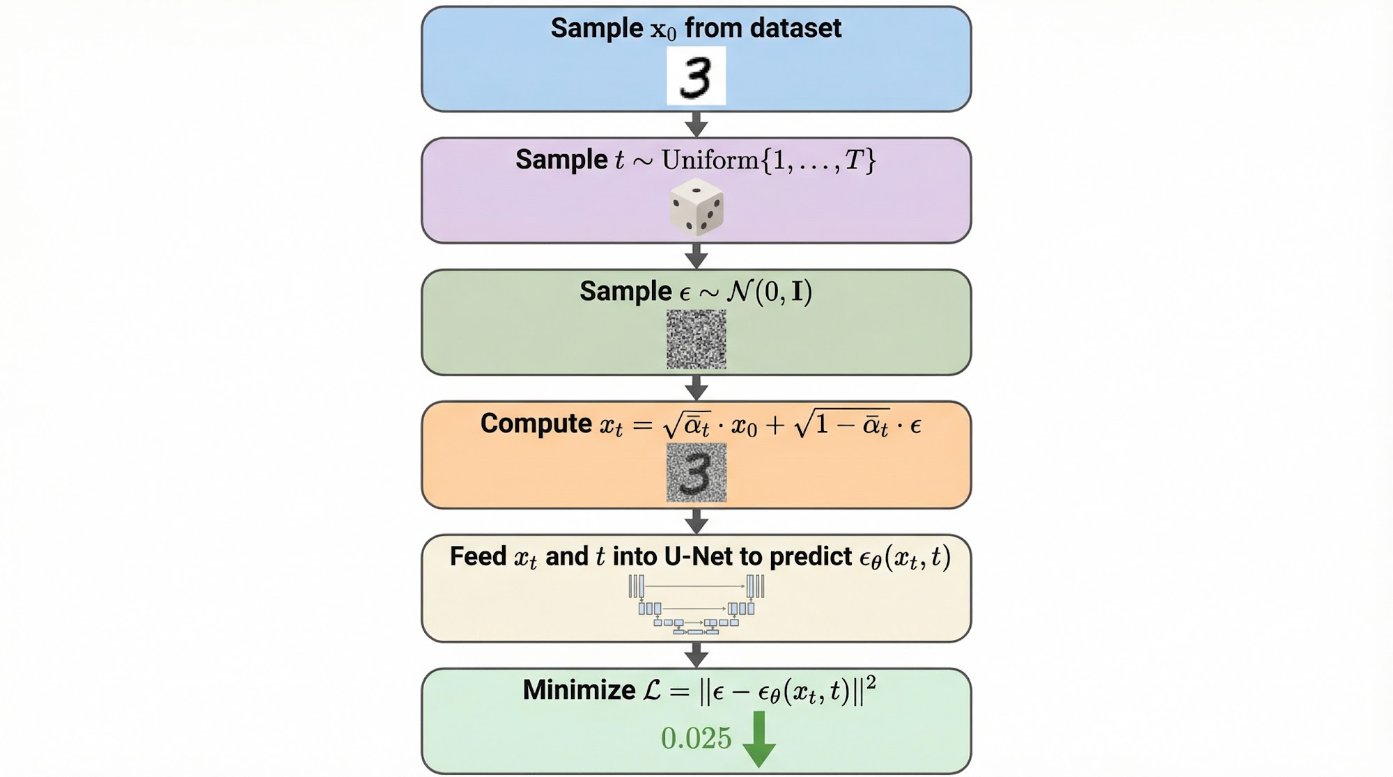
$\mathbf{x}_0 = \frac{1}{\sqrt{\bar{\alpha}_t}} \left(\mathbf{x}_t - \sqrt{1 - \bar{\alpha}_t}\, \boldsymbol{\epsilon}\right)$

If we substitute this into the true posterior mean and reparameterize the model to predict the noise $\boldsymbol{\epsilon}_\theta(\mathbf{x}_t, t)$ instead of the mean directly, the loss simplifies dramatically to:

L_{\text{simple}} = \mathbb{E}_{t, \mathbf{x}_0, \boldsymbol{\epsilon}} \left[ \left\| \boldsymbol{\epsilon} - \boldsymbol{\epsilon}_\theta(\mathbf{x}_t, t) \right\|^2 \right]

This is the final DDPM training objective, and it is remarkably simple: train the network to predict the noise that was added to the image.

Let us plug in numbers to see why this works. Suppose we added noise $\epsilon = 0.3$ to a pixel, and our network predicts $\epsilon_\theta = 0.25$ . The loss for this pixel is $(0.3 - 0.25)^2 = 0.0025$ . If the network perfectly predicts the noise, the loss is zero. The network learns to look at a noisy image at any noise level and figure out exactly what noise was added. This is exactly what we want.

epsilon - epsilon_theta(x_t, t)||^2" with a green loss value shown. Vertical arrows connecting each step. White background. || The DDPM training algorithm distills to six simple steps.

epsilon - epsilon_theta(x_t, t)||^2" in large text, labeled "DDPM Loss: Predict the noise". Downward arrows between boxes with annotations "Same variance -> KL becomes MSE" and "Reparameterize: predict noise instead of mean". A green checkmark next to the bottom box. White background. || The DDPM loss simplifies from a complex variational bound to simple noise prediction.

The U-Net Architecture — The Noise Predictor

Now that we know what to train, the question is: What neural network do we use?

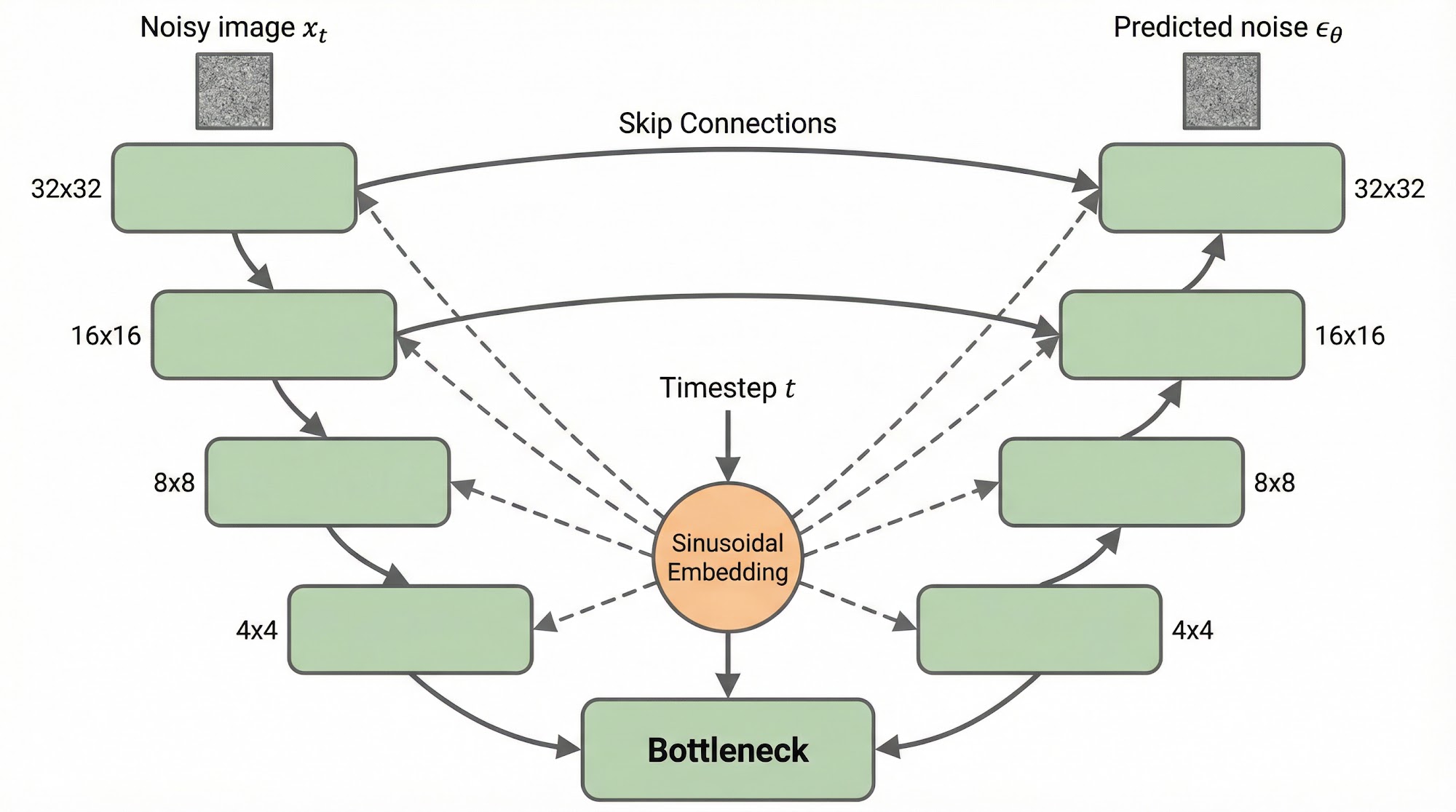
The DDPM paper uses a U-Net architecture, which was originally designed for image segmentation. The U-Net is an excellent choice for this task because it processes images at multiple resolutions while preserving fine spatial details through skip connections.

The U-Net has three main components:

Encoder (downsampling path): A series of convolutional blocks that progressively reduce the spatial resolution while increasing the number of channels. This captures high-level features.
Decoder (upsampling path): A series of convolutional blocks that progressively increase the spatial resolution back to the original size. This reconstructs the spatial details.
Skip connections: Direct connections between encoder and decoder layers at the same resolution. These allow the decoder to access fine-grained spatial information that would otherwise be lost during downsampling.

There is one additional input that the U-Net needs: the timestep $t$ . The model must know which noise level it is denoising, because the denoising strategy at $t = 900$ (very noisy) is very different from $t = 100$ (mostly clean). The timestep is encoded using sinusoidal position embeddings — the same technique used in Transformers — and injected into each layer of the network.

The U-Net takes a noisy image and timestep as input and predicts the added noise.

Sampling — Generating Images from Noise

Now let us understand how we generate images once the model is trained.

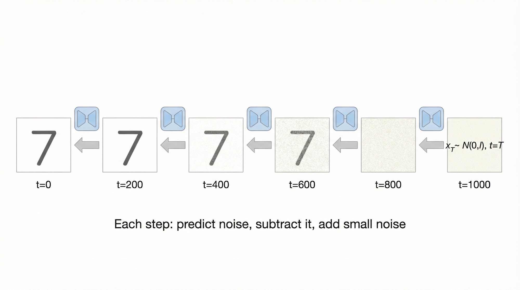
The sampling process starts from pure Gaussian noise $\mathbf{x}_T \sim \mathcal{N}(\mathbf{0}, \mathbf{I})$ and iteratively denoises it for $T$ steps. At each step, the model predicts the noise, and we use this prediction to compute a slightly less noisy image.

The sampling update rule is:

\mathbf{x}_{t-1} = \frac{1}{\sqrt{\alpha_t}} \left(\mathbf{x}_t - \frac{\beta_t}{\sqrt{1 - \bar{\alpha}_t}}\, \boldsymbol{\epsilon}_\theta(\mathbf{x}_t, t)\right) + \sigma_t \mathbf{z}, \quad \mathbf{z} \sim \mathcal{N}(\mathbf{0}, \mathbf{I})

where $\sigma_t = \sqrt{\beta_t}$ and $\mathbf{z}$ is set to $\mathbf{0}$ at the final step ( $t = 1$ ).

Let us walk through what happens at a single step. Suppose we are at step $t = 500$ , with $\alpha_t = 0.99$ , $\beta_t = 0.01$ , $\bar{\alpha}_t = 0.5$ , and a pixel value $x_t = 0.4$ . The network predicts noise $\epsilon_\theta = 0.3$ . We also sample $z = 0.1$ from a standard Gaussian.

The denoised pixel is:

$x_{t-1} = \frac{1}{\sqrt{0.99}} \left(0.4 - \frac{0.01}{\sqrt{1 - 0.5}} \times 0.3\right) + \sqrt{0.01} \times 0.1$

$= \frac{1}{0.995} \left(0.4 - \frac{0.01}{0.707} \times 0.3\right) + 0.1 \times 0.1$

$= 1.005 \times \left(0.4 - 0.00424\right) + 0.01$

$= 1.005 \times 0.3958 + 0.01 = 0.3978 + 0.01 = 0.408$

The pixel moved slightly from 0.4 to 0.408. Each step makes a small adjustment, and over 1000 steps, these small adjustments accumulate to transform pure noise into a clean image.

The full sampling algorithm can be written as:

Sample $\mathbf{x}_T \sim \mathcal{N}(\mathbf{0}, \mathbf{I})$
For $t = T, T-1, \ldots, 1$ $t = T, T - 1, \dots, 1$ :
- Predict $\boldsymbol{\epsilon}_\theta(\mathbf{x}_t, t)$ using the U-Net
- Compute $\mathbf{x}_{t-1}$ using the update rule above
- If $t = 1$ , set $\mathbf{z} = \mathbf{0}$ (no noise at the final step)
Return $\mathbf{x}_0$

One important thing to note: sampling requires $T$ forward passes through the neural network (typically $T = 1000$ ). This makes DDPM sampling relatively slow compared to other generative models like GANs. Later works such as DDIM (Denoising Diffusion Implicit Models) address this limitation by enabling sampling in far fewer steps.

Sampling iteratively denoises pure noise into a clean image over T steps.

Practical Implementation

Enough theory — let us look at some practical implementation now. We will implement the core components of DDPM in PyTorch.

Setting up the noise schedule and forward process:

import torch
import torch.nn as nn
import torch.nn.functional as F

# --- Noise Schedule ---
T = 1000  # Total number of diffusion steps
beta_start = 1e-4
beta_end = 0.02

# Linear beta schedule
betas = torch.linspace(beta_start, beta_end, T)
alphas = 1.0 - betas
alpha_bars = torch.cumprod(alphas, dim=0)

def forward_diffusion(x_0, t, noise=None):
    """Add noise to x_0 at timestep t using the closed-form formula."""
    if noise is None:
        noise = torch.randn_like(x_0)

    sqrt_alpha_bar = torch.sqrt(alpha_bars[t]).view(-1, 1, 1, 1)
    sqrt_one_minus_alpha_bar = torch.sqrt(1 - alpha_bars[t]).view(-1, 1, 1, 1)

    # x_t = sqrt(alpha_bar_t) * x_0 + sqrt(1 - alpha_bar_t) * noise
    x_t = sqrt_alpha_bar * x_0 + sqrt_one_minus_alpha_bar * noise
    return x_t, noise

Let us understand this code in detail. We first define a linear beta schedule from $10^{-4}$ to $0.02$ over 1000 steps. The alpha_bars are the cumulative product of all the alphas, which gives us $\bar{\alpha}_t$ at each step. The forward_diffusion function uses our closed-form formula to jump directly to any noise level — no iteration needed.

The simplified training loop:

def train_step(model, x_0, optimizer):
    """One training step of DDPM."""
    batch_size = x_0.shape[0]

    # Sample random timesteps for each image in the batch
    t = torch.randint(0, T, (batch_size,), device=x_0.device)

    # Sample random noise
    noise = torch.randn_like(x_0)

    # Create noisy images using the forward process
    x_t, _ = forward_diffusion(x_0, t, noise)

    # Predict the noise using the U-Net
    predicted_noise = model(x_t, t)

    # Simple MSE loss between true noise and predicted noise
    loss = F.mse_loss(predicted_noise, noise)

    # Backpropagation
    optimizer.zero_grad()
    loss.backward()
    optimizer.step()

    return loss.item()

This is the entire training procedure! For each batch of images, we sample random timesteps, add the corresponding amount of noise, and train the network to predict the noise. The loss is simply the mean squared error between the true noise and the predicted noise. That is all there is to it.

The sampling loop:

@torch.no_grad()
def sample(model, image_shape, device):
    """Generate new images by iteratively denoising from pure noise."""
    # Start from pure Gaussian noise
    x = torch.randn(image_shape, device=device)

    for t in reversed(range(T)):
        t_batch = torch.full((image_shape[0],), t, device=device, dtype=torch.long)

        # Predict the noise at this step
        predicted_noise = model(x, t_batch)

        # Compute the denoised image
        alpha_t = alphas[t]
        alpha_bar_t = alpha_bars[t]
        beta_t = betas[t]

        # Mean of p(x_{t-1} | x_t)
        x = (1 / torch.sqrt(alpha_t)) * (
            x - (beta_t / torch.sqrt(1 - alpha_bar_t)) * predicted_noise
        )

        # Add noise for all steps except the last one
        if t > 0:
            noise = torch.randn_like(x)
            x = x + torch.sqrt(beta_t) * noise

    return x

The sampling loop starts from pure Gaussian noise and runs the reverse process for $T = 1000$ steps. At each step, the model predicts the noise, we subtract the scaled noise prediction from the current image, and we add a small amount of fresh noise (except at the final step). After 1000 iterations, we get a clean generated image.

Results and Analysis

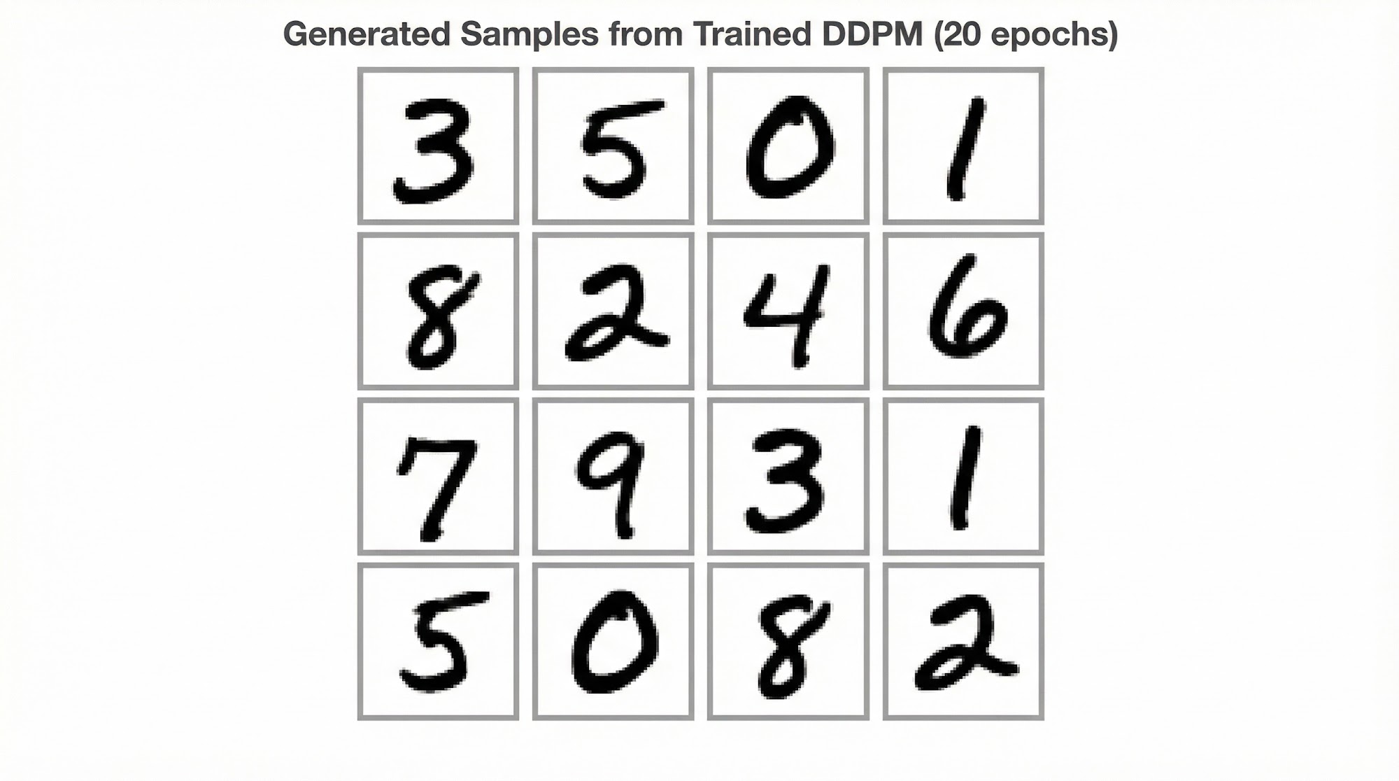
Let us look at the results of training a DDPM on the MNIST dataset of handwritten digits.

After training for approximately 20 epochs, the model learns to generate diverse and realistic handwritten digits.

DDPM generates diverse, high-quality handwritten digits after training.

The progressive denoising process is particularly fascinating to visualize. We can see how the model gradually builds structure from nothing:

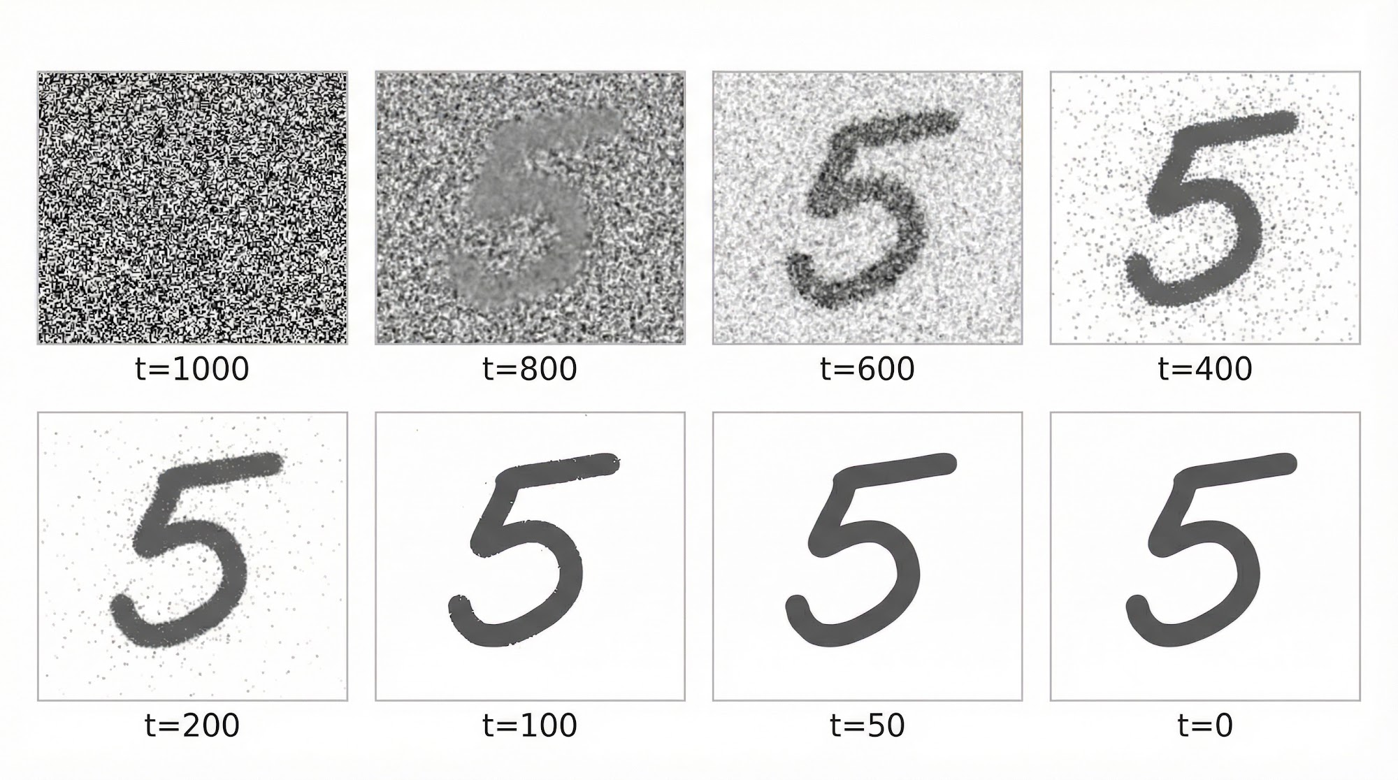
The model progressively removes noise to reveal a clean image during sampling.

We can see that in the early denoising steps (high $t$ ), the model makes large-scale structural decisions — deciding the rough shape and position of the digit. In the later steps (low $t$ ), the model refines fine details like stroke thickness and sharpness. Not bad right?

Connection to Score-Based Models

Before we wrap up, let us briefly look at an elegant connection. It turns out that DDPM's noise prediction is intimately related to score matching from score-based generative models.

The score function $\nabla_{\mathbf{x}} \log p(\mathbf{x})$ points in the direction of increasing data probability — like a compass pointing toward high-probability regions.

It can be shown that the noise prediction and the score function are related by:

\boldsymbol{\epsilon}_\theta(\mathbf{x}_t, t) = -\sqrt{1 - \bar{\alpha}_t}\; \nabla_{\mathbf{x}_t} \log q(\mathbf{x}_t)

In other words, predicting the noise is equivalent to estimating the score function (up to a scaling factor). This beautiful connection was formalized by Song et al. (2021), who showed that both DDPMs and score-based models can be unified under a single framework of stochastic differential equations.

This means that when our U-Net predicts the noise added to an image, it is simultaneously learning the gradient of the log-probability of the data distribution. The sampling process of DDPM is essentially Langevin dynamics with learned scores. This connection is truly amazing — two seemingly different approaches to generative modeling turn out to be two sides of the same coin.

Wrapping Up

Let us summarize the key ideas of DDPM:

Forward process: Add Gaussian noise gradually over $T$ steps until the image becomes pure noise. A closed-form formula lets us skip to any noise level directly.
Reverse process: Train a U-Net to predict the noise added at each step. The loss is simply $\|\boldsymbol{\epsilon} - \boldsymbol{\epsilon}_\theta(\mathbf{x}_t, t)\|^2$ .
Sampling: Start from pure noise and iteratively denoise over $T$ steps using the trained model.
Connection: Noise prediction is equivalent to score estimation, unifying DDPMs with score-based generative models.

The elegance of DDPM lies in its simplicity — a complex generative model reduces to a straightforward denoising task. This framework has since been extended to produce stunning results in image generation (DALL-E 2, Stable Diffusion, Imagen), audio synthesis, video generation, and even molecular design.

Here is the link to the original paper: Denoising Diffusion Probabilistic Models (Ho et al., 2020)

That's it!