
Your First World Model — MiniPong
We build one thing today, completely and from scratch: a neural network that learns how a small game works — so well that at the end, you can play the game inside the network's imagination. And then we watch, honestly, as that imagination falls apart.
Let us start with the demo, because it is the whole lecture compressed into one image.
We wrote a tiny Pong-like game. We let a random player bash the keys for a while and recorded what happened. Then we trained a neural network on those recordings — and asked it a strange question at every timestep: before the game shows you the next frame, paint what you think it will look like. From the previous frames and the player's key press alone. No access to the game's code, no physics equations, no labels of any kind.
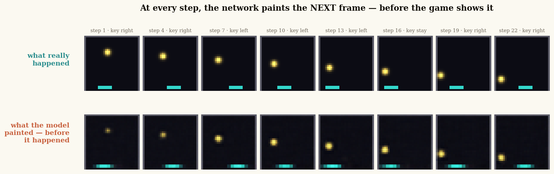
Top row: the real game. Bottom row: the network's painting of each next frame, produced before the game revealed it. Ball position, ball direction, paddle response — all correct, at every step.
Look at the bottom row. Ball position: correct. Ball direction: correct. The paddle responding to the key press: correct. The network learned this world purely from recorded play. That is a world model — the subject of this entire series, now sitting in front of you as a working artifact instead of a definition.
Let us be equally precise about what today is not. There is no controller, no planner, no reward, no reinforcement learning. The machinery for acting well in a world comes later in the series. Today has a single question, and we will answer it completely: how does a network learn a world?
Here is the whole plan on one picture. Part 1 is training: collect episodes, compress frames into codes with one network, learn to predict the next code with a second network that carries a memory. Part 2 is deployment: switch the game off, run the trained model in a closed loop, feed it your key presses — and play inside it.
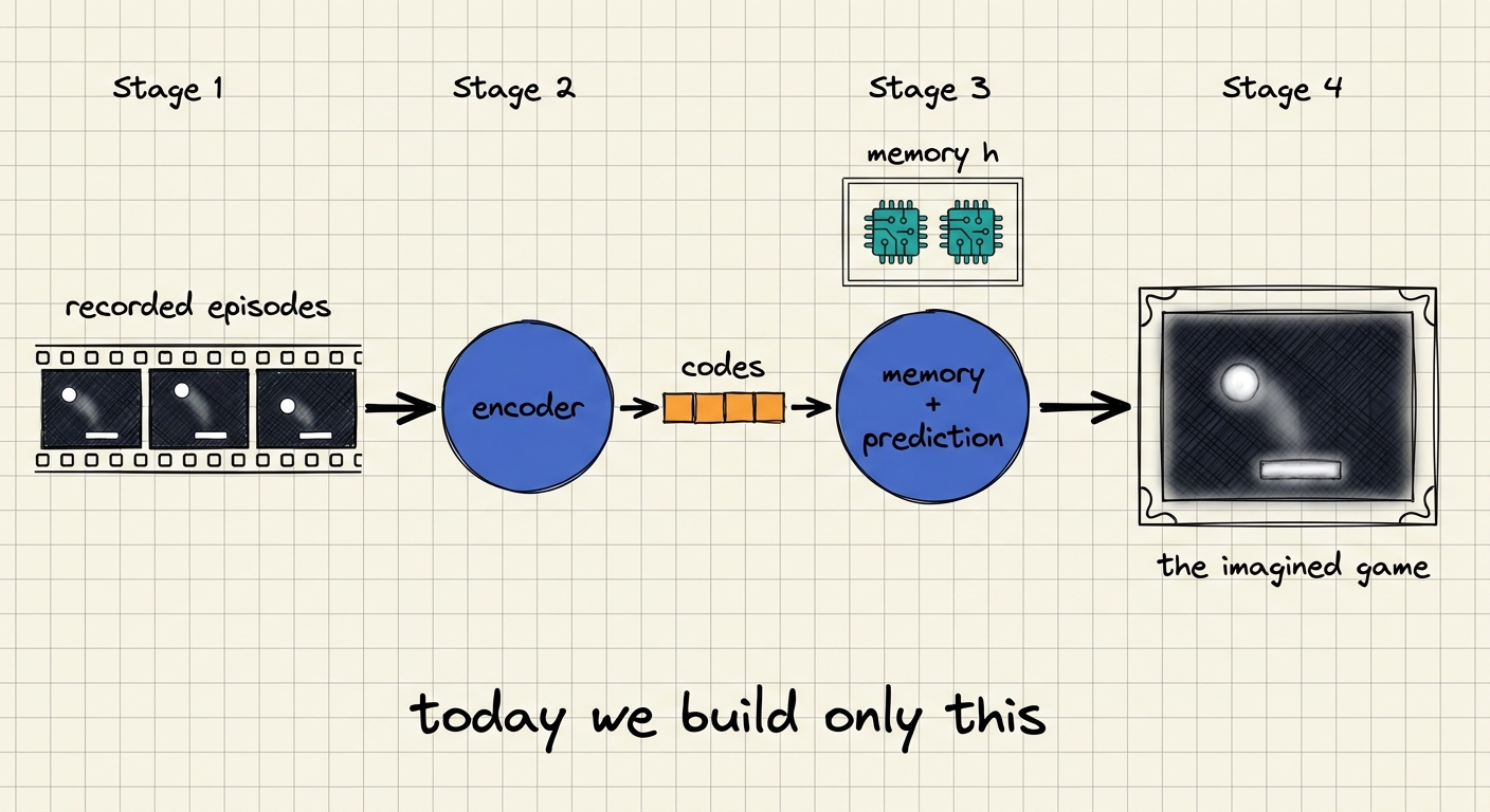
The full pipeline. Training on the left: episodes → codes → memory → prediction. Deployment on the right: the same networks, running in a closed loop with no game engine behind them.
The World: MiniPong
Our world for today is a small Pong-like game we wrote in about 60 lines of Python. It has exactly three properties you need to hold in your head.
The screen is 32 × 32 pixels with 3 colour channels, so every frame is 32 × 32 × 3 = 3,072 numbers.
The objects are a paddle at the bottom that you move with 3 actions — left, stay, right — and a ball that flies one pixel per step, bounces off the walls, and bounces off the paddle, which can bend its direction.
The catch — and remember this, because it will shape the entire architecture — is what a single frame cannot tell you. Look at any one frame: you can see where the ball is. You cannot see where it is going. Velocity is invisible in a snapshot.

Eight raw observations from MiniPong. Everything the model will ever know about this world enters through frames like these.
Why such a small world? Because we want to see everything. Every tensor, every loss value, every failure will be inspectable, and the entire build — data collection, both networks, all experiments — runs in under ten minutes on a laptop CPU. When something breaks (and something will break, twice, in instructive ways), we will be able to say exactly why.
The Dataset: 24,000 Frames of Random Play
A world model learns from experience, so first we need experience. We let a random player play 200 episodes of 120 timesteps each. At every timestep we store exactly two things: the frame (what the screen showed) and the action taken. Total: 200 × 120 = 24,000 frame–action pairs. Nothing else — no labels, no rewards, no object positions.
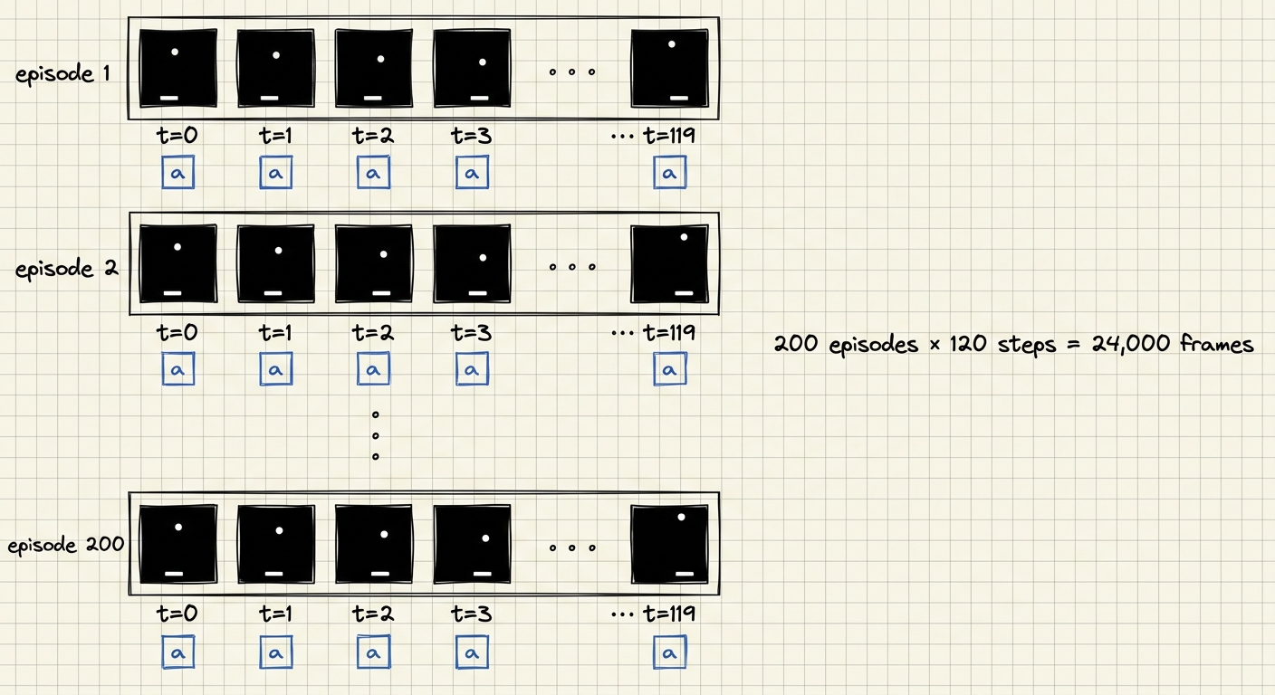
Each episode is a strip of frames paired with the actions taken. This raw experience is the only teacher the model will ever have.
Why a random player? Because the world model's job is to learn how the world works — and physics does not care whether the player is skilled. The ball bounces the same way for a champion and for a cat walking on the keyboard.
There is one subtlety worth internalizing, because it is the kind of detail that separates builds that work from builds that mysteriously don't: our random player holds each key for a while before switching, the way a human would, rather than resampling a fresh action every frame. At deployment, a human player holds keys too. Training data must visit the situations deployment will visit — a model trained only on frantic frame-by-frame jittering has never seen what happens when the paddle glides steadily left for ten steps.
Network V: Compressing the World into Twelve Numbers
A frame is 3,072 numbers, but the situation is tiny: a ball position and a paddle position. So the first network, V, is an encoder–decoder. The encoder squeezes each frame into a code z of just 12 numbers; the decoder proves nothing important was lost by redrawing the full frame from the code alone. We train it on all 24,000 frames with one signal: make the redrawn frame match the original.
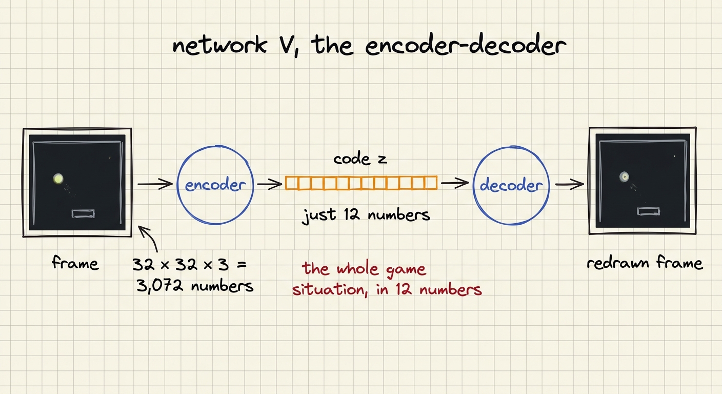
The encoder–decoder. Everything the prediction machinery will ever manipulate is the 12-number code at the waist.
Two training details matter enormously later, so let us name them now. First, during training we add a little noise around each code before decoding. Why? Because soon another network will predict codes, and its predictions will land near real codes, never exactly on them — and a point near a code must still decode to a sane frame. Second, consecutive frames are pushed to get nearby codes: the world moves smoothly, so the code space must move smoothly too.
We trained V — 332 seconds on a laptop CPU — and immediately hit our first honest lesson.
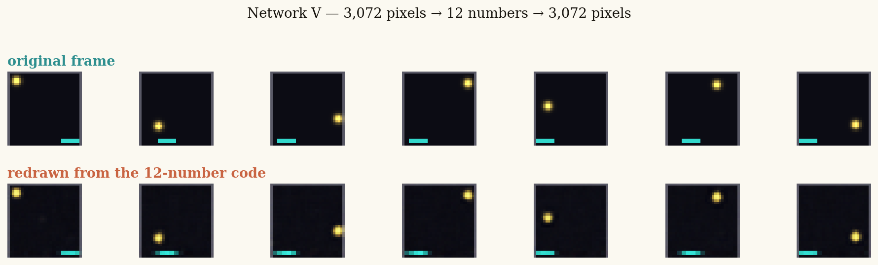
V's report card: held-out frames redrawn from their 12-number codes. But our first attempt at this figure had no ball in the bottom row at all.
Our first V redrew the paddle perfectly and completely dropped the ball. Why? The ball is 4 bright pixels out of 1,024. To a plain reconstruction loss, ignoring it costs almost nothing — the network gets 99.6% of the pixels right by painting the paddle and the background and pretending the ball does not exist. The fix is one line: weight the bright pixels more heavily in the loss, so the smallest, most dynamic object on screen becomes the most expensive thing to get wrong.
Burn this into memory, because you will meet it in every world model you ever build: compression keeps what the loss pays for — nothing else. The most important object in a scene is often the smallest one, and no loss function knows that unless you tell it.
Why One Frame Is Never Enough
Now we want to predict the next frame. Here is where the catch from earlier comes due.
The current frame alone cannot tell us what happens next. The ball at position (12, 9) might be moving down-left or down-right — both situations look identical right now. The information we need — velocity — lives in the difference between consecutive frames, not in any single one.
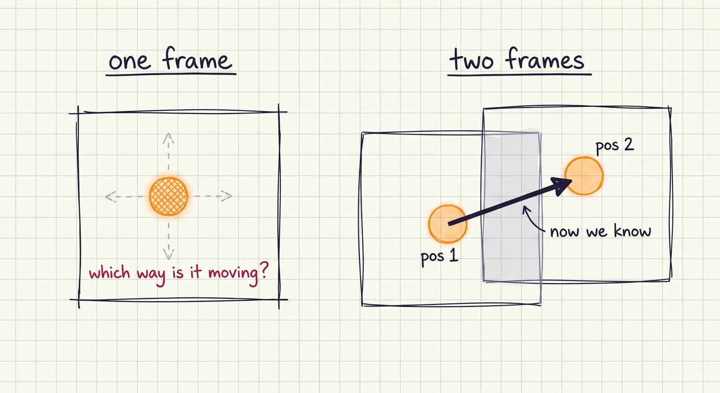
The same frame, two incompatible futures. No function from one frame to the next frame can be correct — the input does not contain the answer.
The consequence is the single most important design decision of the lecture: the prediction network cannot be a simple frame-in, frame-out function. It needs a memory — a vector that persists across timesteps and accumulates what single frames cannot show.
Network M: A Memory That Discovers Velocity
The memory in our build is a GRU carrying 128 numbers. At every timestep it takes three inputs — the memory as it was, the current code z, and the action a — and produces the updated memory. That is the entire update rule.
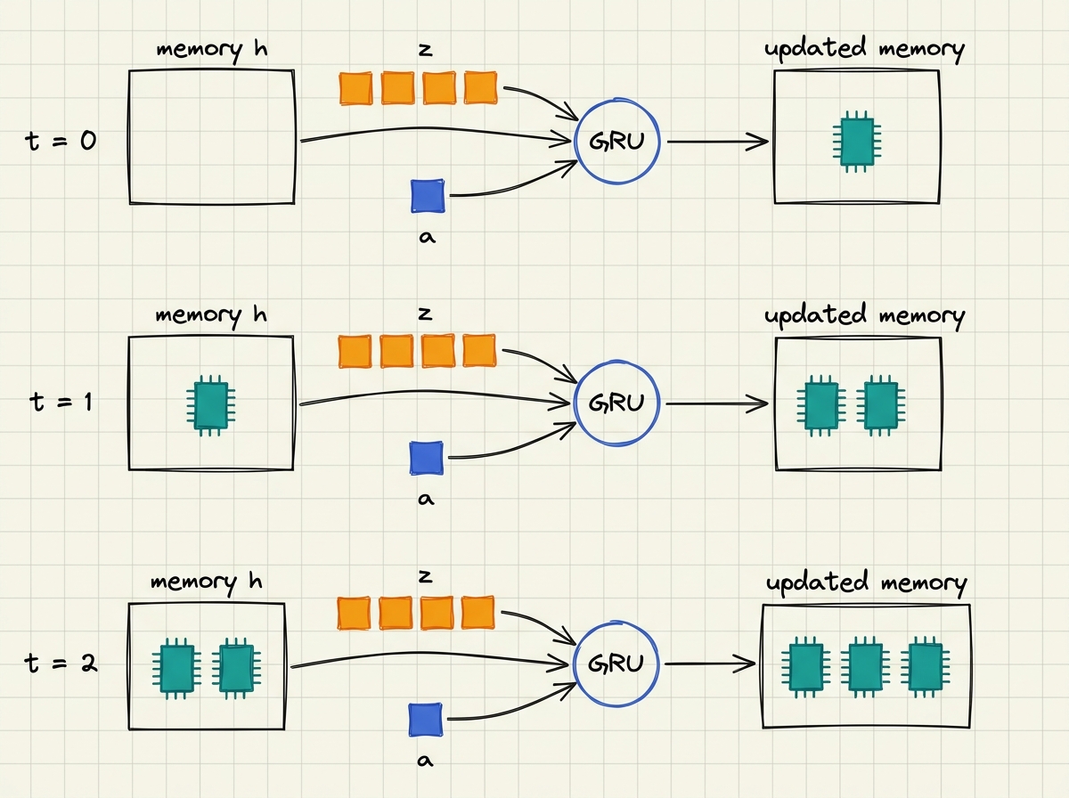
Read it row by row. At t = 0 the memory is empty. After one step it holds where things are. After two steps it holds the fact no frame ever showed: which way the ball is moving.
Read the figure row by row and watch what the memory can know. At t = 0 it is empty. After one step it holds one fact: where things are. After two steps it holds the fact that no single frame ever showed — which way the ball is moving — because it has seen two positions and can keep their difference. The memory is never wiped during an episode; only rewritten.
Now let us pin down the bookkeeping precisely, because this is where every learner's questions live. At timestep t = 5 the model reads three things: the code of frame 5 (from network V), the action taken at step 5, and its own memory, which has digested steps 0 through 4. It must then output a guess for the code of frame 6 — a frame it has not seen. Frame 6's real code, computed by V, is the answer key.
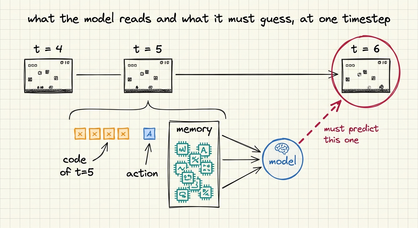
The exam at one timestep. This repeats at every timestep of every episode: 24,000 small exams.
And here is the full training step, the heart of the entire lecture. Network 1 (the GRU) blends memory + code + action into the updated memory. Network 2 (a small two-layer head) reads the updated memory and outputs the predicted next code. The real next frame goes through V to give the actual next code. The loss is the distance between predicted and actual — and its gradient trains both networks together, at every timestep, across all 200 episodes, epoch after epoch.
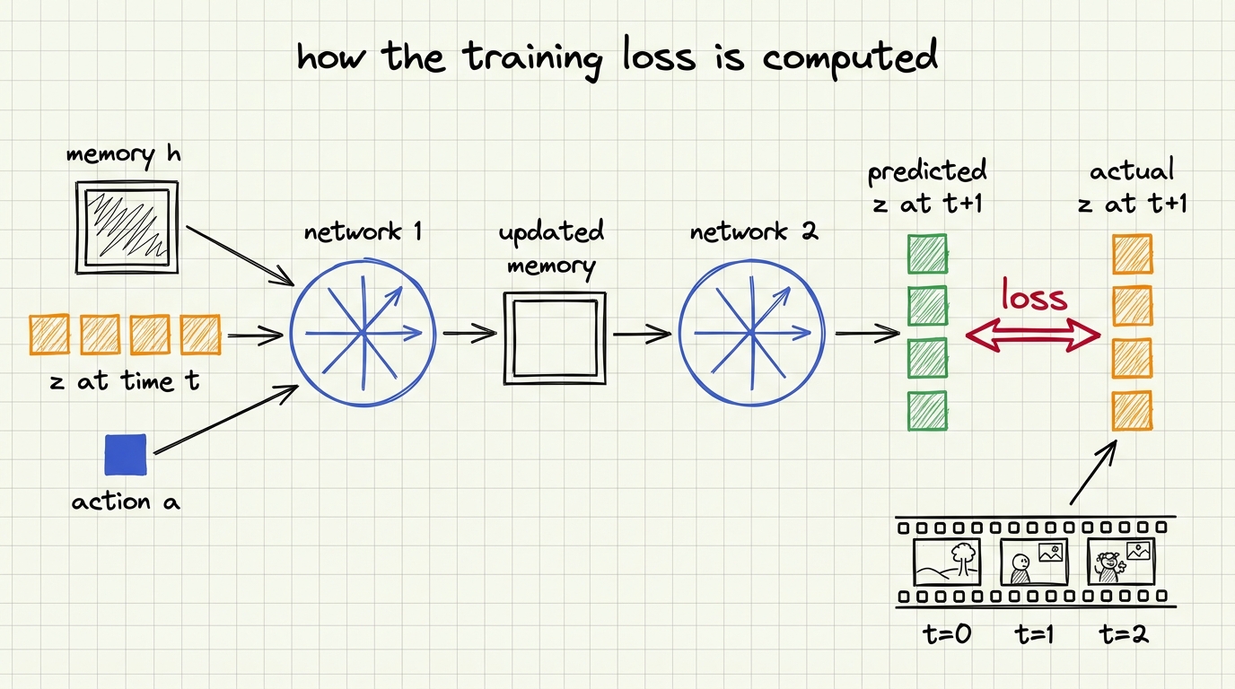
Prediction (green) versus reality (orange), in code space. One distance, one gradient, two networks trained together. That is how a network learns a world.
That's it. No physics engine, no object detector, no hand-written rules. One loss: predict the next code.
The result that proves the memory story
If the memory story is true, it makes a sharp, testable prediction. Measure the prediction error separately at each timestep of fresh episodes. At t = 1 the error should be large — velocity is unknowable from a single frame, so the model is guessing between down-left and down-right. From t = 2 onward, once the memory has seen two positions, the error should collapse.
We trained M (46 seconds) and ran exactly that experiment.
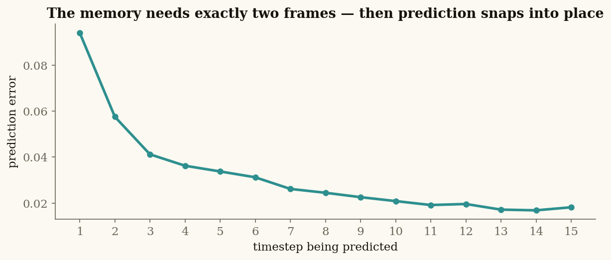
Exactly as the theory predicted: the error is high precisely when the memory cannot yet contain velocity, and snaps down the moment it can.
The error is 0.094 at the first step — then it collapses to 0.041 by step 3 and stays there. Nobody told the network about velocity. It discovered that keeping the difference between two positions is the most useful thing a memory can do, because prediction is what the loss pays for. The same principle that lost us the ball in V's loss now works in our favor in M's.
Two questions you should be asking right now. Why two networks — can't we do it in one? You can: nothing stops you from training a single network that maps (frame, action, memory) → next frame directly. We split it because each piece is reusable and inspectable — V's codes can be studied on their own, and M can be swapped without retraining vision. And a preview: the next lecture merges them back into one jointly-trained model, and shows exactly what that buys. Why squeeze all of history into one vector — why not attention? Excellent instinct: that is precisely what a Transformer would do — keep all past frames and look back at any of them directly. The trade is that attention's memory and compute grow with history length, while the recurrent vector stays constant-size forever. Modern world models use both, and we will meet the attention-based ones later in the series.
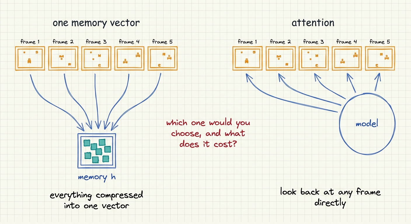
The recurrent memory versus attention over the full history. Constant-size state versus growing lookback — a trade-off that runs through every modern world model.
Deployment: The Model Becomes the Game
Now, the moment the whole build has been pointing at. Switch the game off.
During training, the model received a real frame's code at every step. Now there are no frames — the game engine is gone. So the loop changes in one crucial way: the predicted code is fed back in as if it were real. The player presses a key → the GRU and the prediction head produce the predicted next code → the decoder paints it to the screen → the player sees the painted frame and presses the next key → the prediction becomes the next step's input. Around and around.
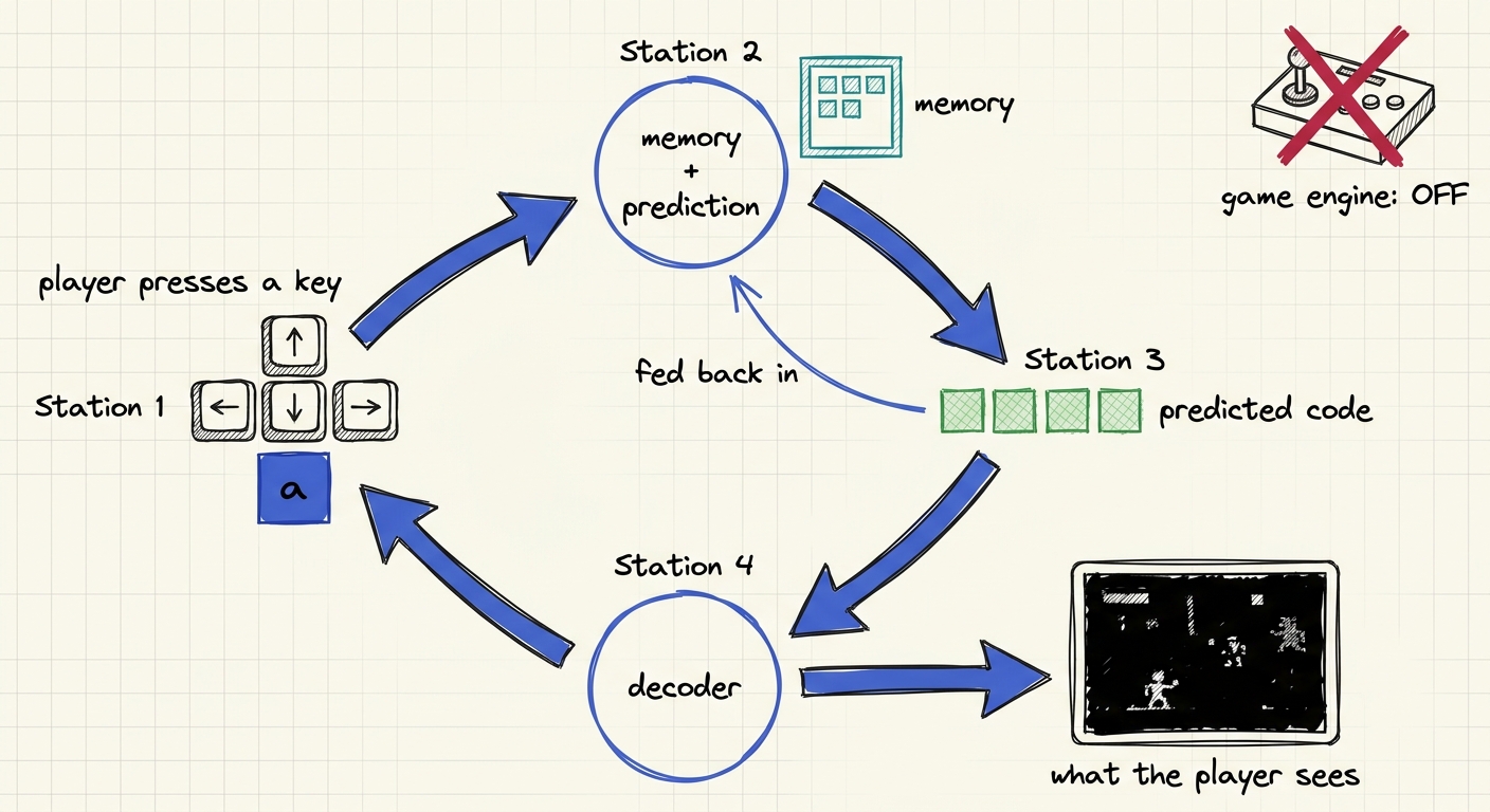
The deployment loop. The model is no longer predicting the game. The model is the game.
Training in open loop and running in closed loop are different sports, and our first deployed model made that painfully clear: the paddle stayed perfect, and the ball was lost within a few frames. Getting a survivable dream took three pieces of honest engineering, in the order we found them.
First, every code dimension must matter equally. The paddle dominates the code's variance, so the training loss barely noticed errors in the dimensions encoding the ball. The fix: normalise each of the 12 code dimensions to the same scale before training M — and keep the bright-pixel weighting in V's loss, or compression happily drops the smallest, most important thing on screen.
Second, practise the closed loop during training. After normal training, fine-tune M on closed-loop rollouts: it must predict several steps ahead while eating its own outputs, with each predicted code decoded back to pixels and compared against the real frame. And predict the change in the code rather than the code itself — when the model is unsure, "nothing moves" is a far safer default guess than "fade everything toward the average".
Third — and this one surprised us — the world itself must be learnable. Two of our "obviously fine" game-design choices were quietly fatal. Random ball respawns: a deterministic predictor facing true randomness predicts the average of all outcomes, which renders as an invisible smear. And integer-pixel motion: positions that snap to whole pixels give the codes isolated islands in code space, and a prediction landing between islands paints nothing. Deterministic physics plus smooth sub-pixel motion fixed both.
The Honest Failure: Watching the Dream Collapse
With all three fixes in place, here is the closed loop for real. Top row: the real engine. Bottom row: the model's imagination, fed the same key presses and its own predictions — not one frame from the game.
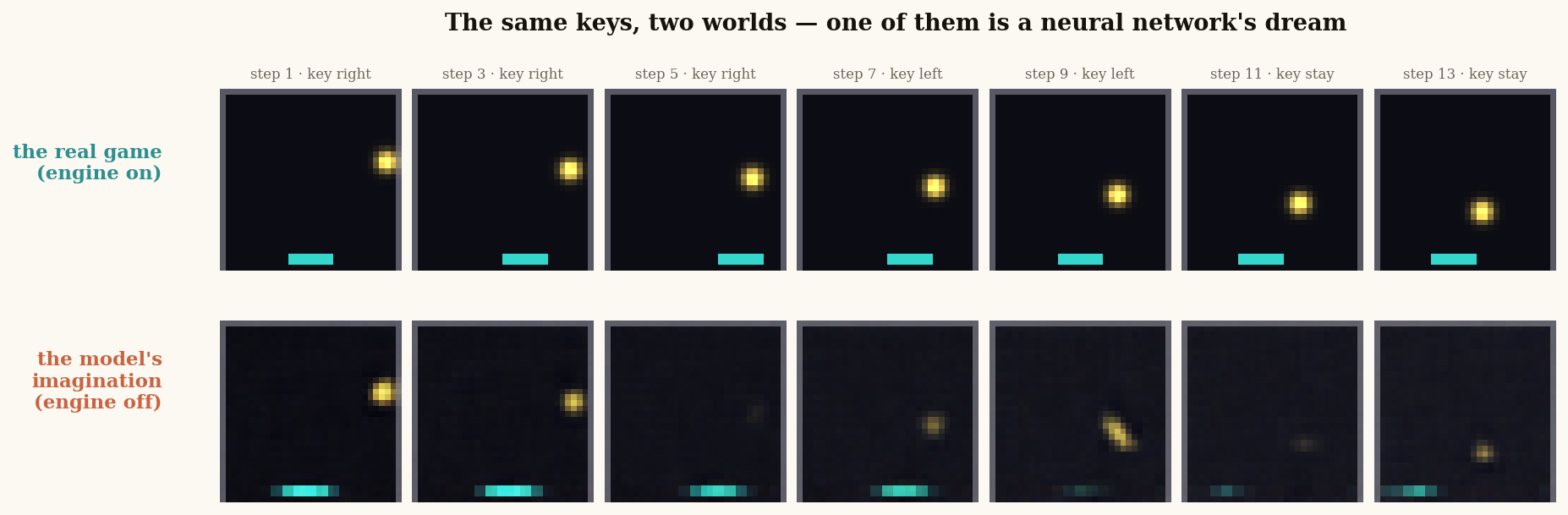
The dream, honestly. The paddle obeys every key for as long as you play. The ball is painted correctly for the first steps — then fades, smears, and re-forms as the dream drifts.
The paddle obeys every key for as long as you care to play. The ball is painted for the first steps — and then it fades, dissolves, and re-forms somewhere else as the dream drifts away from anything the real game would do. Total machinery behind this: two networks, 167,527 parameters, trained in under ten minutes on a laptop.
Why does the dream collapse? Because of an asymmetry we have now seen from both sides. One-step prediction is near-perfect — you saw it in the opening demo. But in a closed loop, every tiny error is eaten as input and amplified at the next step. An error of a fraction of a pixel becomes a slightly wrong code, which becomes a slightly wrong prediction from a slightly wrong starting point, and within a handful of steps the compounding takes the trajectory somewhere the model has never seen. This compounding-error problem is THE central problem of world models — not a bug in our little build, but the fundamental obstacle that every serious world model, from Atari dreamers to robot-learning systems, is engineered around.
And notice why our model is especially vulnerable: V was trained to reconstruct, M was trained to predict, and neither knew about the other. The encoder never knew its codes would be consumed by a predictor eating its own outputs. We trained them separately, and at deployment we paid for it.
Four things to keep from this build:
- A world model = compress + remember + predict. An encoder to a small code, a memory updated every timestep, a head that predicts the next code. Three jobs, two small networks, one loss.
- Compression keeps what the loss pays for. The ball vanished until we made the loss care about it. Watch for this in every model you ever train.
- Memory earns its keep in exactly two frames. Error 0.094 with one frame of history, 0.041 with three — velocity lives in the difference between frames, and the memory learned to keep it unprompted.
- Deployment is a different sport from training. A model that predicts one step well can still collapse when it eats its own predictions. Practise the closed loop; respect true randomness.
Run It Yourself
Everything in this article — every number, every plot — is the real output of one companion notebook, pong_worldmodel.ipynb. It contains MiniPong itself (~60 lines), the dataset collection, network V, network M with the memory, the per-timestep error experiment, and the playable closed loop. It runs end to end in about 8 minutes on a laptop CPU or free Colab, using only numpy, torch, and matplotlib.
Then break it, deliberately — the notebook ends with three exercises, each a one-line change: shrink the code from 12 numbers to 3 and see what breaks first; zero the memory at every step and watch prediction fail exactly where the theory says it must; re-enable random ball respawns and watch the deterministic predictor smear — then explain why.
Next: Dreams That Last
You now own a network that contains a playable copy of its world — and you watched that copy drift when pushed too far. The next question writes itself: how do we make dreams that last?
The diagnosis is already on the table. Our encoder never knew its codes would be used for prediction; we trained V and M separately, then paid for it in the closed loop. The fix is the RSSM — the Recurrent State-Space Model — which trains compression and prediction together, as one model built from the ground up for long, stable rollouts. That is the next lecture in this series, "Dreams That Last", taught on the Vizuara YouTube channel — and you can go one step further and train an RSSM on real robot data in the Dreams That Last build in the Production Lab at /projects/robot-dreams.
First we learned the world. Next we make the dream hold.