
The Journey of a Token Through a World Model
A picture-word enters a trained IRIS transformer as the single integer 99. Something leaves the top of the stack that can name the next word. This is the full story of what happens in between — traced, not drawn, on a real model.
A quick recap before we open anything up. IRIS is a world model built like a language model. A VQ-VAE tokenizer — trained first, then frozen — compresses each 64×64 game frame into 16 integers drawn from a 512-word codebook. A causal transformer is then trained on those integers, interleaved with the actions the player took, and its entire job is to predict the next token: given everything so far, which of the 512 words comes next? It never sees a pixel. Sample a word, append it, repeat sixteen times, hand the sixteen words to the decoder, and you have imagined the next frame. In the previous pod we built this pipeline on CoinRun and watched it dream. We called the middle component "a transformer" and moved on.
That is the what. It is not enough to actually understand the model. So this pod is the how, at full detail, on the model we trained. One rule makes it worth your time: everything here is traced, not drawn. One real forward pass, on a held-out CoinRun episode — every heatmap, every number, every attention bar below is read straight out of the trained network.
The question is simple to state. A word enters the stack as the integer 99. Something leaves the top that can name the next word. What happened in between?
First, the shape of our model, so the numbers mean something: 136 positions, 256 numbers per position, 6 layers, 8 heads each, a 512-word output. About 6.9 million parameters. Small enough to print, big enough to be real.
Section 1: The Whole Stack, Before We Walk It
Here is the entire journey on one page. Read it bottom to top: tokens enter at the bottom, a probability over 512 words leaves at the top, and everything in between is the same block, repeated six times. The rest of this article walks up this diagram one step at a time.
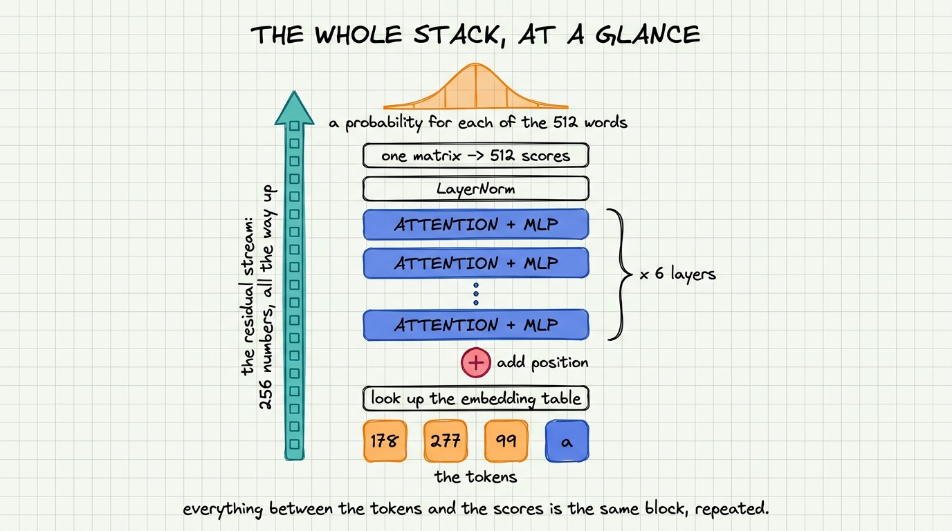
The whole stack: everything between the tokens and the scores is the same block, repeated six times.
Four things organize everything that follows. First, every position keeps its own 256 numbers the whole way up — 136 positions in, 136 out, no pooling, no bottleneck. The stack is 136 parallel lanes that occasionally exchange information. Second, only one operation ever moves information between lanes: attention. Everything else — the MLP, the normalisations — works on one position at a time and cannot see its neighbours. Third, the block is identical every time: six layers means the same shape six times over, with different weights. Learn one block and you have learned the network. Fourth, only the last lane is asked a question. All 136 positions produce an output, but when we imagine, we read exactly one of them — the last — and ignore the rest.
Section 2: What the Transformer Is Actually Handed
The input is not an image, and it is not a frame. It is a flat stream of 136 integers: eight frames, each contributing sixteen picture words plus one action token. Eight times seventeen is 136 positions. This stream is the only thing the model sees — there is no image and no recurrent memory anywhere in it.
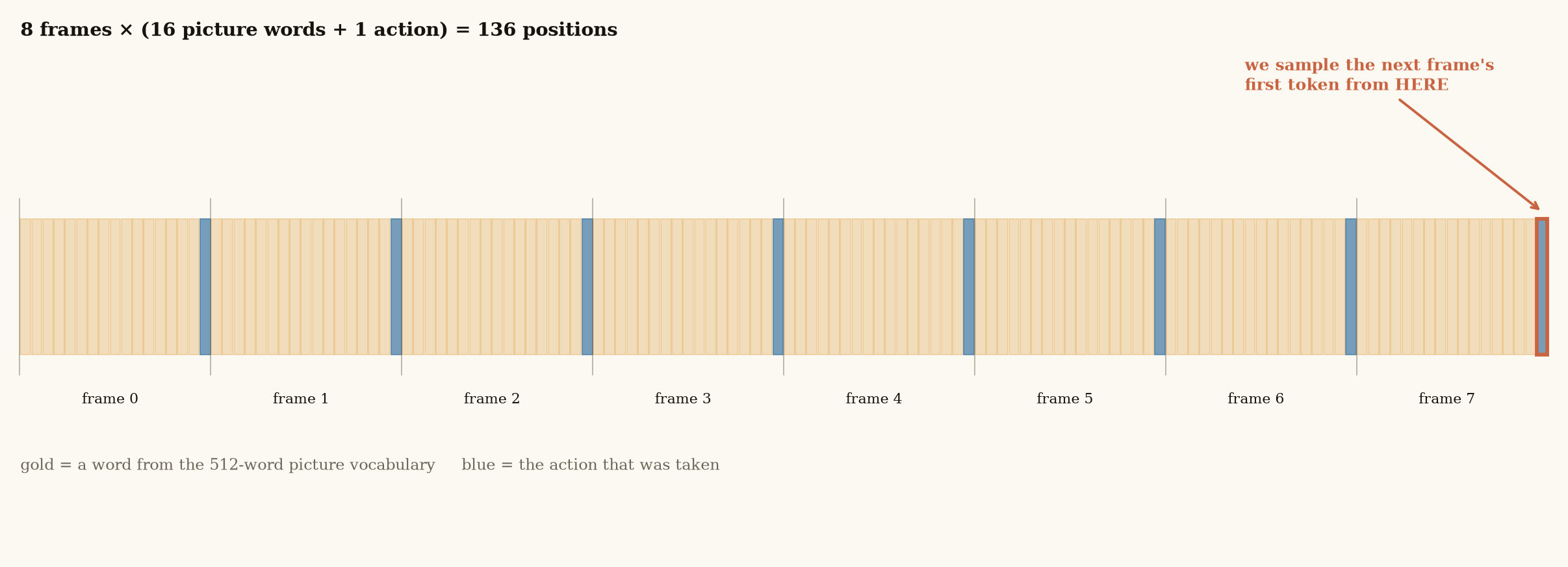
Eight frames × (sixteen picture words + one action) = 136 positions. This flat stream is everything the model sees.
Three decisions are already baked into that picture. A frame is not one thing — it is sixteen. Each frame contributes sixteen separate positions in a fixed raster order, so the model can attend to part of a past frame — the patch where the player was, and nothing else — which a single pooled frame embedding would never allow. The action is a token like any other: not a side input, not a conditioning vector, but a seventeenth position with its own embedding table. This is precisely why the same architecture works unchanged for text, video and control.
And the position we care about is the last action token. Its output predicts the first word of the next frame. Everything in this article traces that one position. Get its loss mask wrong and the model can finish a frame but never start one — which is a mistake we actually made while building this.
Section 3: The Integer Becomes a Vector — and It Is Not the Codebook Vector
Here is the single most common misunderstanding about IRIS, so let us be blunt about it. The tokenizer's codebook stores a 64-number vector for word 99. It is natural to picture that vector sliding out of the VQ-VAE and into the attention stack. That is not what happens.
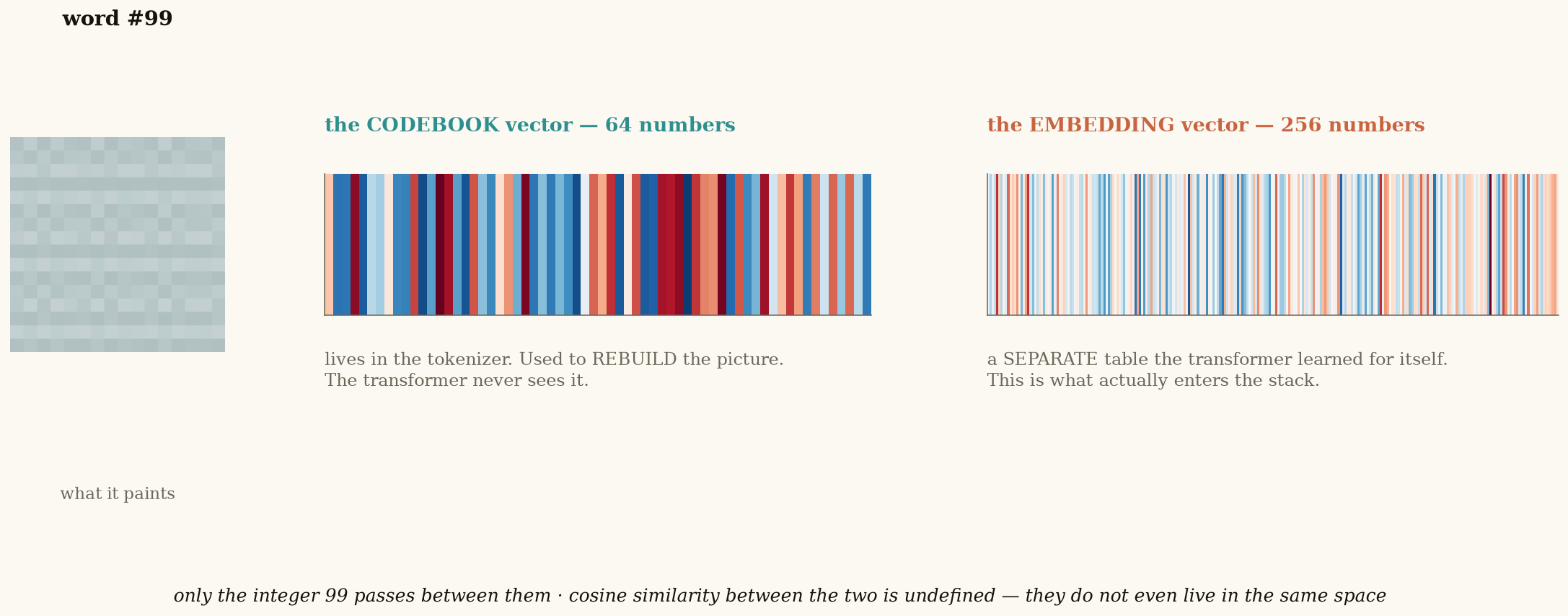
The tokenizer's codebook vector and the transformer's embedding are two different objects for the same word, joined only by the integer.
The tokenizer's job ends at the integer. Encode, snap to the nearest codebook entry, emit 99. The 64-number codebook vector exists so the decoder can repaint the patch — that is its only job. The transformer keeps its own dictionary: a separate 512 × 256 embedding table, learned from scratch during dynamics training. Word 99 looks up its row of that table.
And this is exactly what a language model does. The characters "c-a-t" are not a vector; cat is token 5372, and GPT looks up row 5372 of its own table. The two halves of IRIS are joined by an integer, which is precisely why the tokenizer can be frozen and the transformer trained on top of it.
"Look up the embedding" sounds like a database query; it is simpler than that. The table is a 512 × 256 matrix of ordinary weights — one row per word, 131,072 parameters trained by gradient descent exactly like every other weight in the network. The lookup selects row 99 and copies it out. That is the entire operation. (Formally it is a one-hot vector times the matrix, which is why gradients flow back into exactly one row per occurrence.)
The consequence is worth pausing on: the model chooses what its own words mean. At the start of training these rows are random — word 99 means nothing. They acquire meaning only because the loss pushes words that behave alike toward similar rows. The vocabulary was given by the tokenizer; the meanings are the transformer's own.
Section 4: The Position Table That Discovered the Number 17
There is a problem with what we have built so far. Attention computes a weighted sum, and a sum does not care about order — shuffle the input positions and you get the same answer. That would be fatal for a world model: "player left, then right" and "player right, then left" would be indistinguishable.
So position is added to the vector. A second learned table, one row per slot in the window, is added straight onto the word embedding. Position 0 and position 135 get different rows, so the same word in two places becomes two different vectors. Note what this costs: the table has exactly 136 rows, so the model cannot be shown a longer window without learning new ones. The RSSM of Lecture 4 had no such limit — this is the first real price of keeping the past instead of summarising it.
Now for the first of the two discoveries. Here is the position table our model actually learned, along with the similarity between every pair of position vectors.
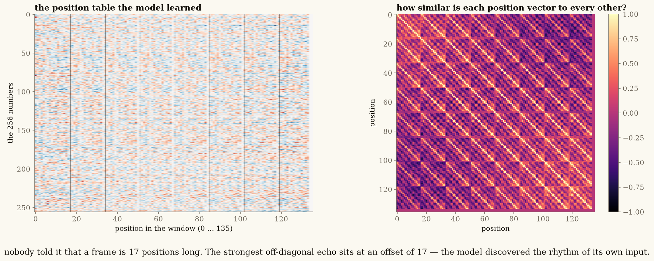
The actual learned table, and the similarity between every pair of positions — the strongest off-diagonal echo sits at an offset of exactly 17.
The position table starts as 136 rows of zeros. No sine waves, no hand-designed structure — just free parameters. Whatever pattern is in there was put there by the loss. And it grew a period of 17: positions 17 apart end up with the most similar vectors of any offset beyond ten. Seventeen is exactly one frame — 16 picture words plus one action. Nobody told the model that. It worked out the rhythm of its own input from nothing but next-token prediction, because "I am the 3rd patch of a frame" is a genuinely helpful thing to know when you are predicting the 4th. A caution worth keeping: this is one small model on one game — a nice demonstration that structure can be learned rather than imposed, not evidence that it always is.
The other structural ingredient at this stage is the causal mask — a 136 × 136 triangle that decides who may look at whom.
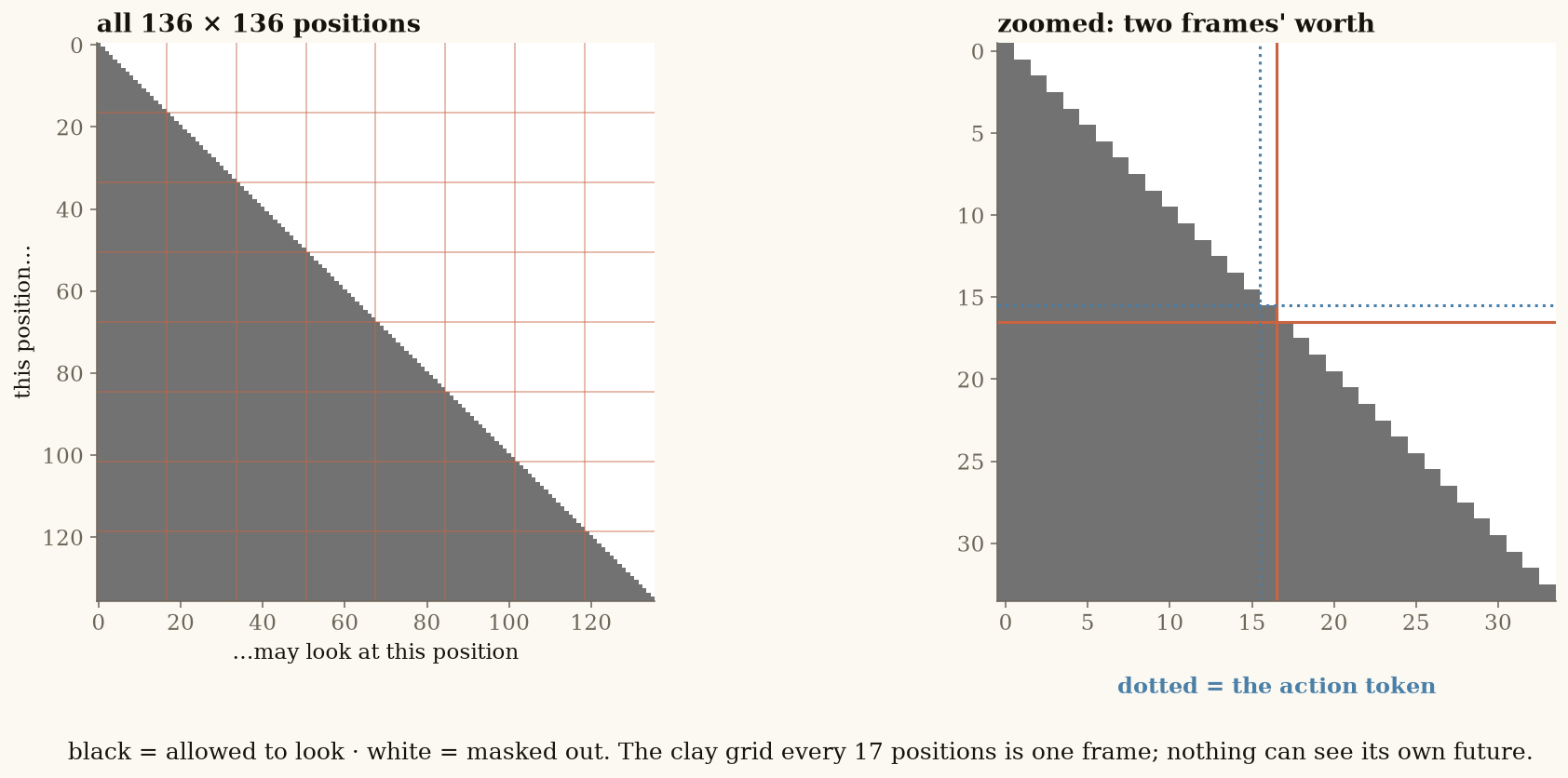
Black = allowed to look, white = masked out. The grid marks every 17th position, where one frame ends and the next begins; the dotted line marks the action token whose output predicts the next frame's first word.
This triangle is why transformers train fast. Without it, the model would cheat: position 40 predicting position 41 while being allowed to look at position 41 learns nothing. With it, every position trains at once — one forward pass produces 136 honest predictions, each conditioned only on its own past, and every one can be scored, because during training the correct answers are already on disk. An RNN would need 136 sequential steps to do the same work.
One asymmetry worth naming now: this parallelism is a training property. When we imagine, there is no future to feed in — we are inventing it — so we run the stack, sample one word, write it into the sequence, and run the whole stack again. Sixteen passes per imagined frame. Same weights, same mask, completely different cost.
Section 5: Attention — Three Questions, Eight Heads
Now the only operation that moves information between lanes. Every position holds one 256-number vector, and three separate matrices turn it into three different vectors, each with a different job.
The query asks: "what am I looking for?" It is built from the position doing the asking — here, the last action token, about to predict the next frame's first word. The key answers: "what do I have on offer?" It is built from every position that might be looked at, and the dot product of a query with a key is the match score — big when they point the same way. The value says: "and here is what you get if you pick me" — a third vector carrying the content actually handed over. The output is the values, blended in the softmaxed proportions.
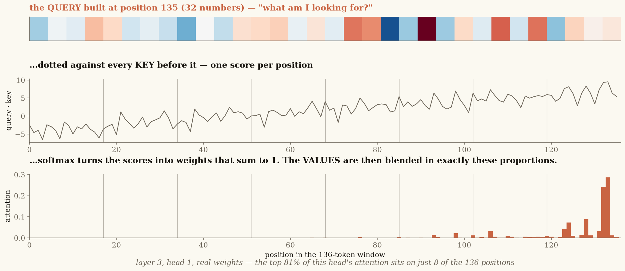
Layer 3, head 1, traced from the trained model: a query is built, dotted against every key before it, and softmaxed into weights that sum to one.
One small detail decides whether the thing trains at all: the scores are divided by √32 before the softmax. Without that, the dot products grow with dimension, the softmax saturates, and gradients vanish.
And attention does not happen once per layer — it happens eight times, in parallel, and not as eight copies of the same thing. Each head gets 32 of the 256 dimensions: one attention, carved into eight independent 32-dimensional subspaces. Same cost, more expressiveness. The reason you want more than one head is that a single softmax sums to one — pointing hard at the patch above forces the head to give up looking at the patch to the left. With eight heads you can do both at once.
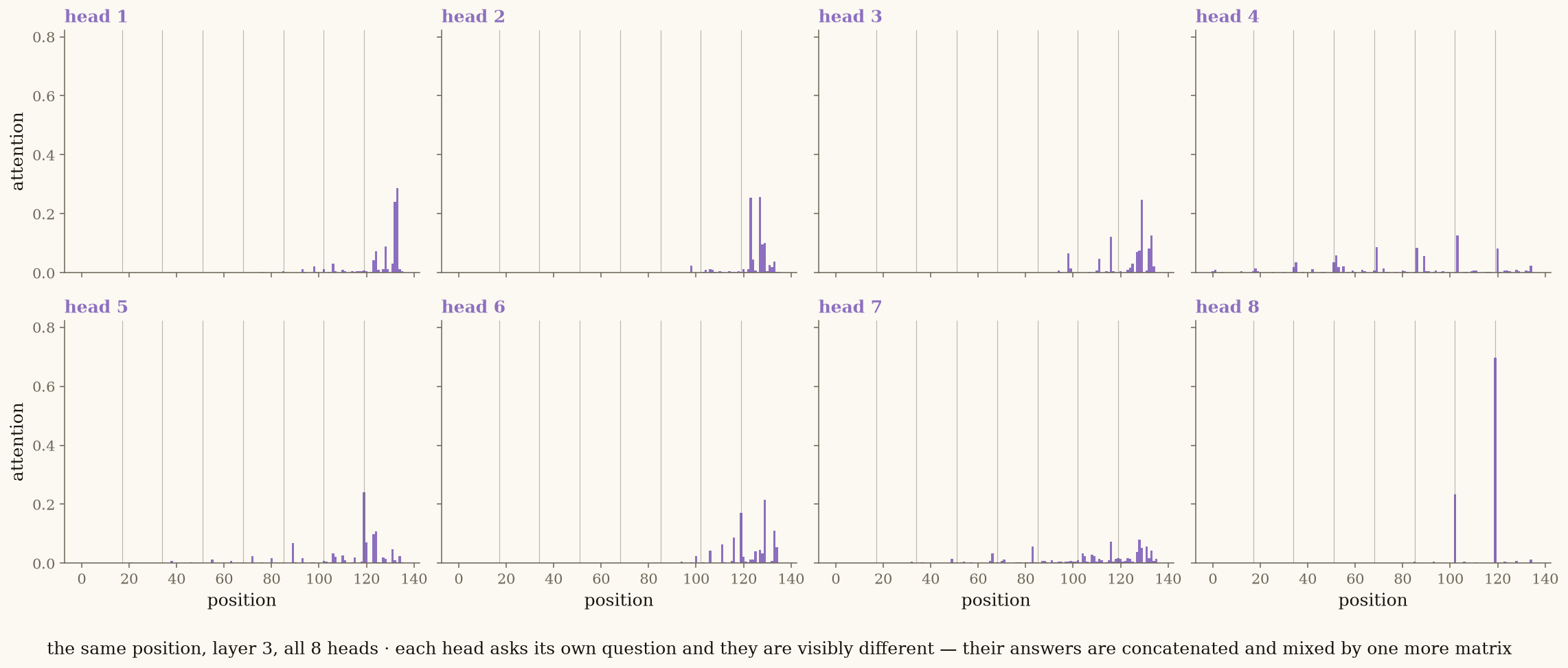
The same position, all eight heads of one layer, read from the trained model — they are visibly not doing the same job.
Then they are stitched back together: the eight 32-number results are concatenated back into 256 and passed through an output matrix that decides how to combine them. That is the complete attention sublayer.
Section 6: The Anatomy of a Block, and the Residual Stream
Attention is only half of a block. Here is the whole thing.
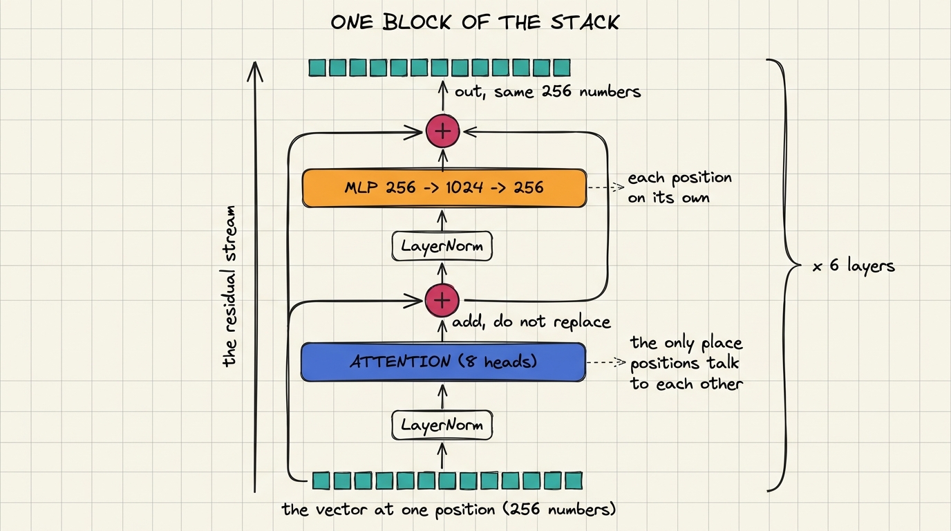
One block: normalise, attend, add the result back in; normalise, MLP, add the result back in. This shape repeats six times.
The other half is a two-layer MLP — 256 → 1024 → 256 with a nonlinearity — applied to each position on its own. The division of labour is clean: attention moves information; the MLP processes it. Attention is a weighted average, so it can only ever gather; the MLP is where the gathered information is turned into something new — and two thirds of the model's parameters live there. Crucially, the MLP sees one position at a time, every position processed by the same small network independently. All communication between positions happens in attention and nowhere else.
But the most important wire in the diagram is the one that looks like it does nothing: the residual connection. Each sublayer adds its result to the running vector rather than replacing it. The stream is never overwritten.
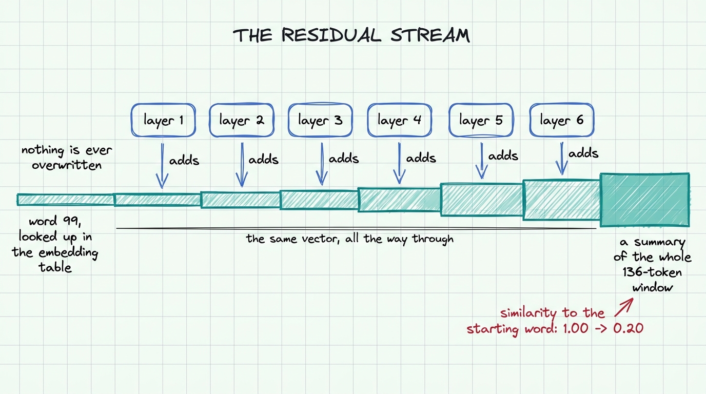
The vector at one position is never replaced — every sublayer adds to it. What arrives at the top is the input embedding plus twelve corrections.
This is why six layers can be stacked at all. Because the stream is never overwritten, a gradient can reach layer 1 directly — and each layer only has to learn a correction, not the whole answer. What arrives at the top is the input embedding plus twelve added refinements (two per block). One more convention: we normalise before each sublayer, not after — pre-norm — which makes deep stacks trainable without a learning-rate warm-up, and is what almost everything modern does.
So what does this stream actually do to our token? Here it is, measured on our model — one position, traced through all six layers.
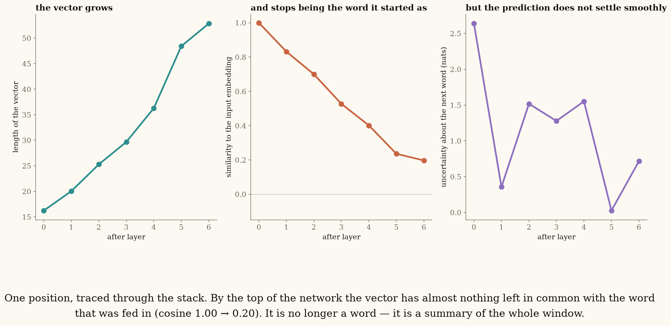
One position traced through all six layers: it always has 256 numbers; what changes is their magnitude (16.2 → 52.8) and what they mean (similarity to the starting word 1.00 → 0.20).
This is the measurement the whole lecture was built for. The thing people call "the context vector" is not produced by a special mechanism — it is this stream, at the last position, after the last layer. Three things happen to it on the way up.
It starts as one word and ends as a summary: cosine similarity to its own input embedding falls from 1.00 to 0.20. By the top of the stack there is almost nothing left of "word 99" — it has been overwritten, by addition, with information pulled from the other 135 positions.
It gets bigger, not longer. The vector always has exactly 256 numbers; that never changes. What grows is its magnitude, from 16.2 to 52.8, because each layer adds more into the stream than it cancels. The vector accumulates rather than transforms.
And every position is doing this simultaneously. There is no single context vector — there are 136 streams running side by side, each summarising its own past. We only read the last one because that is the one being asked a question.
Section 7: What the Layers Divided Between Themselves
If each layer adds a correction, do the layers add the same kind of correction? We can measure that: at each layer, take the attention from the sampling position and ask what share of it falls inside the newest frame.
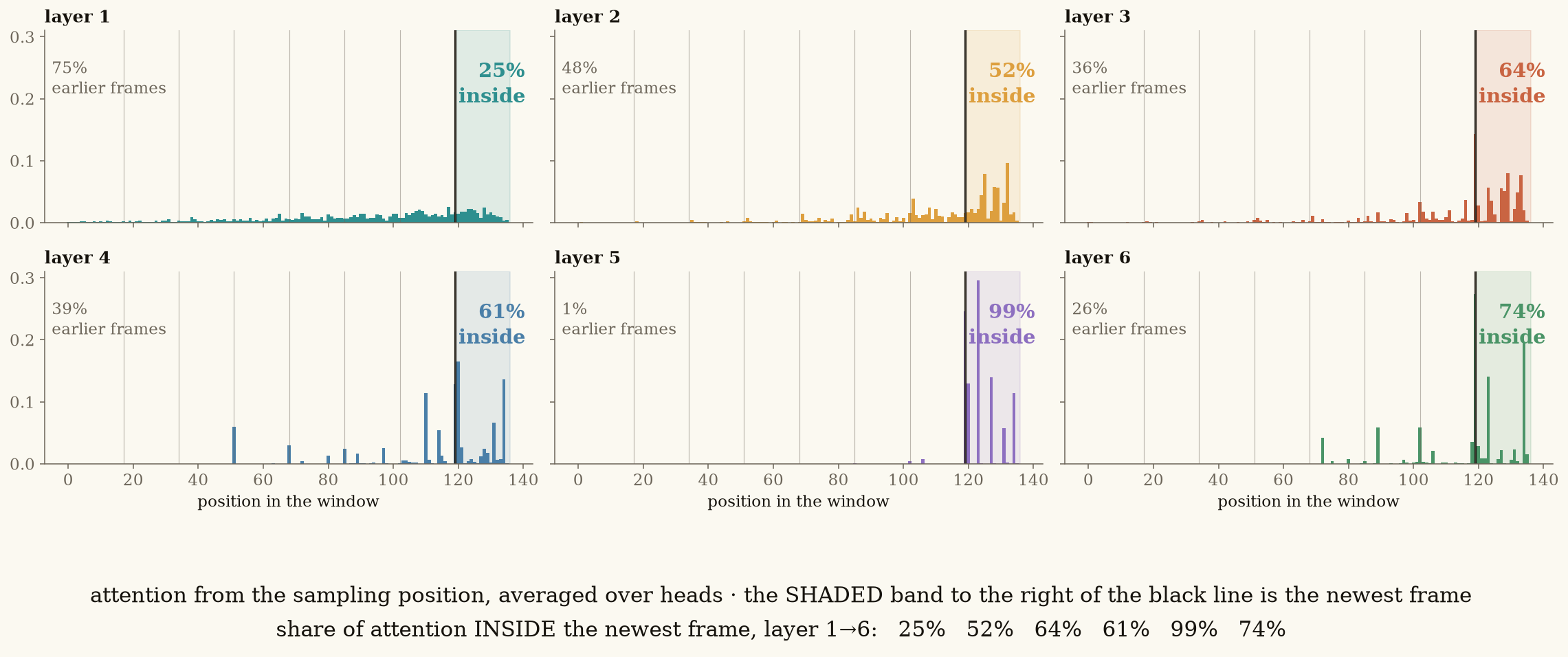
Layer 1 → 6, the share of attention on the newest frame: 25% · 52% · 64% · 61% · 99% · 74%. Early layers reach back across history; later ones settle onto the frame being finished.
Layer 1 spends three quarters of its attention on the past — only 25% inside the newest frame. It is gathering context: where the player was, which way things were moving. Layer 5 puts 99% on the current frame — by then the context has already been folded into the stream, and the upper layers are doing local work: given everything I now know, what belongs in this patch? Gather low, decide high. Nobody designed that split; the loss did. It is a pattern you will see again and again in transformers — with a fair warning: this is one position, on one episode, in a small model. Evidence, not a law.
The residual stream buys us one more trick, and it is a good one: you can decode the middle of the network. Because the stream is never replaced, an intermediate vector lives in the same space as the final one — so you can take the output head, trained only for the top, and point it at layer 3. Nothing stops you. This is known as the logit lens.
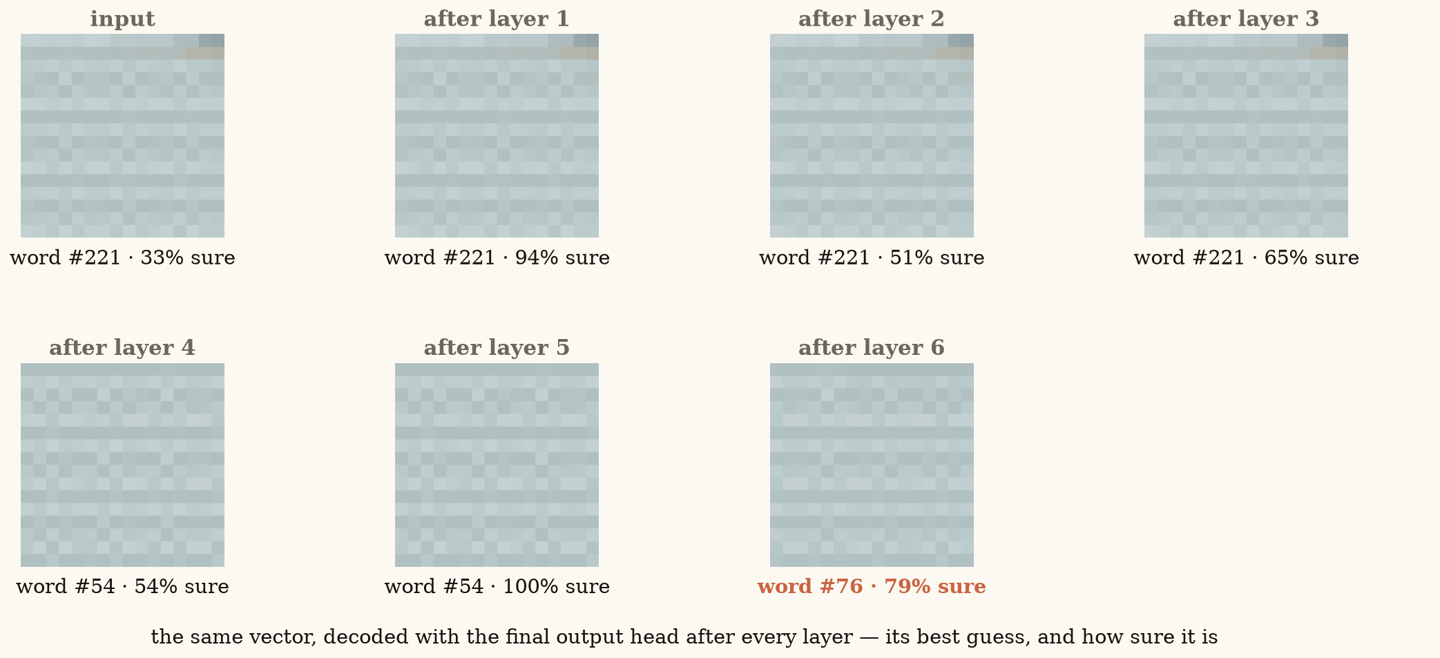
The same vector, decoded with the final output head after every layer: its best guess is word 221 for four layers, flips to 54, and lands on 76. The answer is assembled on the way up, not looked up.
The guess changes twice: 221 → 221 → 221 → 221 → 54 → 54 → 76. The network does not know the answer early and refine it; it changes its mind, late. Confidence does not rise smoothly either — uncertainty falls, spikes, and falls again. "Deeper = more certain" is a story we tell; the measurement does not support it. And note that this interpretability trick only works because of the residual: in a network where each layer replaced its input, layer 3's vector would live in a private space and the final head would read noise.
Section 8: Out of the Top — a Probability for Every Word
At the top of the stack: one final normalise, then one matrix maps the 256-number vector to 512 scores, and a softmax turns them into a probability for every word in the vocabulary.
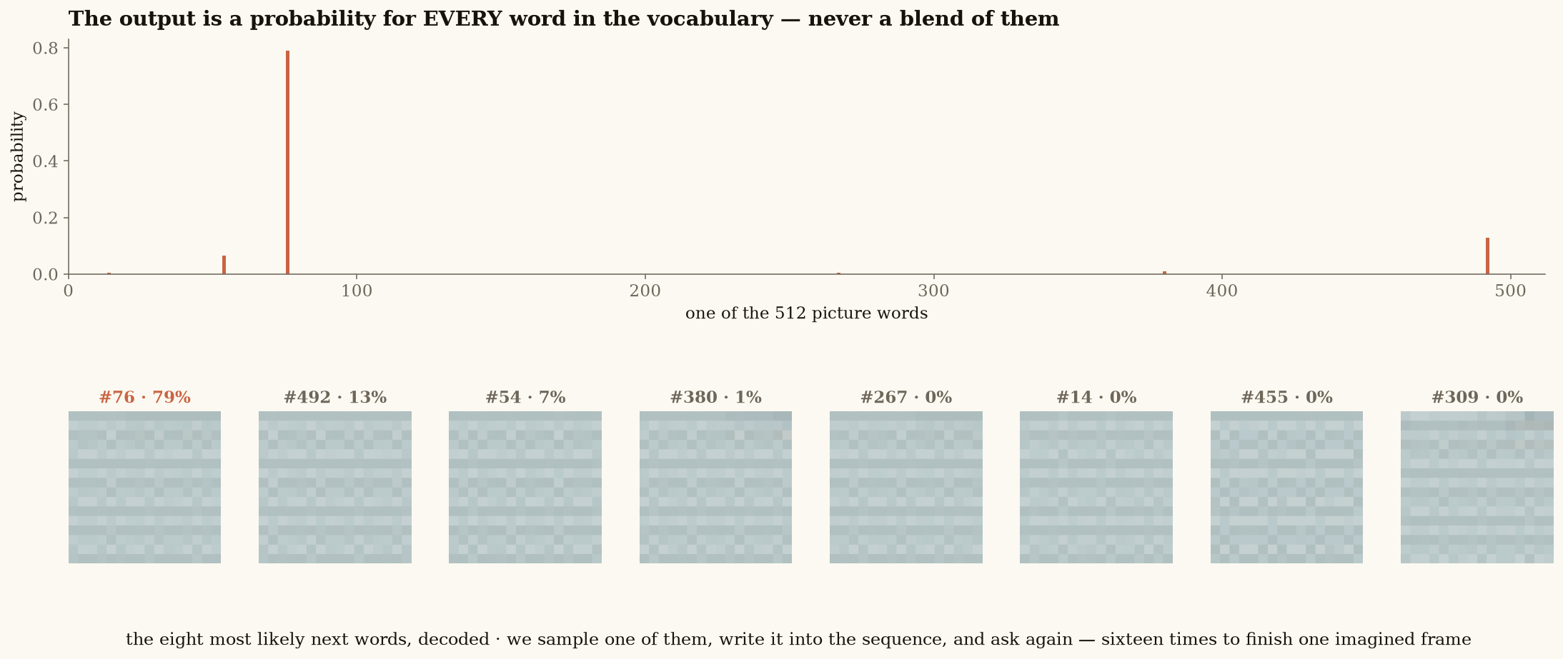
Word 76 at 79%, word 492 at 13%, word 54 at 7% — three genuinely different continuations, each a real picture.
Look at that distribution carefully, because it is the payoff of the whole discrete-latent design. The model is genuinely unsure between three different-looking patches — and it says so, by naming all three. Each candidate is a word that exists, a real patch the decoder can paint. A Gaussian head could not have done this: it would have had to output one point, and the point between three different patches decodes to exactly the blur we diagnosed in the RSSM's dreams. This one output layer is why the lecture was called "a vector or a vocabulary".
Then we sample one word, write it into the sequence, and run the whole stack again — sixteen times for one imagined frame. That loop is the world model.
Here is the entire journey, once more, in nine steps:
- A frame becomes sixteen picture words, plus one action — 136 integers in the window.
- Each integer looks up the transformer's own embedding — 136 × 256.
- A learned position vector is added — 136 × 256.
- Six times: normalise, then attend under the causal mask — 8 heads × 32 dimensions.
- Six times: add the attention result back into the stream.
- Six times: normalise, MLP 256 → 1024 → 256, add back.
- A final normalise.
- One matrix to vocabulary size, then softmax — 136 × 512.
- Sample the last position; repeat sixteen times for a frame.
That is the entire model. 6.9 million parameters, no recurrence, no hidden state carried between steps — and the "memory" is nothing more than the fact that the old tokens are still sitting in the window. The integer 99 went in knowing only its own name; what came out the top was a 256-number summary of everything in the window, sharp enough to put 79% of its probability on the right next word. Sixteen matrices later, a word became a world.