A Vector or a Vocabulary?

Every world model we have built so far carried its knowledge as a handful of continuous numbers. IRIS asks a different question: what if the model carried words instead — and read its own past the way a language model reads a sentence?

Section 1: The Dream You Can Drive

Let us start with the demo, because it is the destination of everything in this pod.

Two world models watch the same eight real frames of CoinRun — a procedurally generated platformer where a small character runs, jumps, and collects a coin. Then the screen goes off. No game engine is running anymore. You press left, right, or jump, and each model imagines the next frame — frames that have never existed anywhere. Press a different button and you can watch the futures separate: at step one the imagined branches differ in just 2 of 16 tokens; by step six, in 14 of 16. Every branch was rolled out on a GPU ahead of time — 3,279 real rollouts — so the whole thing runs offline, on your laptop.

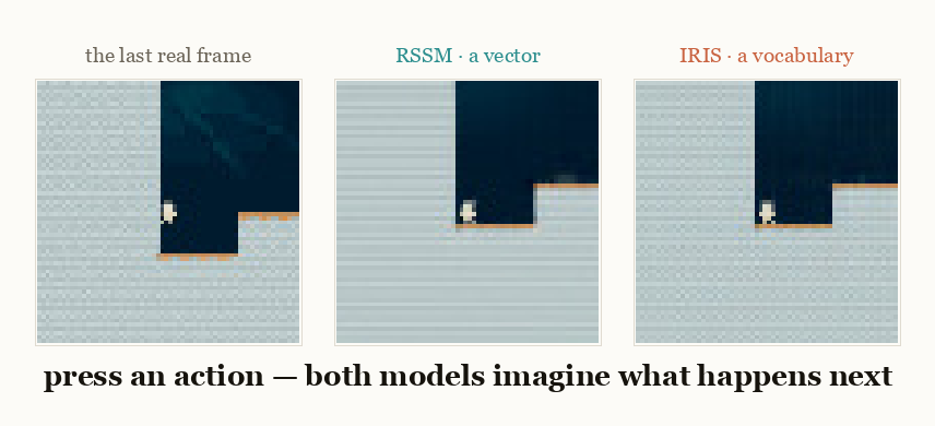
The dream simulator: the last real frame, and what each world model imagines happens next for the action you chose.

By the end of this pod you will understand every number on that screen. The lecture it is built from was taught on the Vizuara YouTube channel as part of the Build a World Model from Scratch series, and every figure and measurement here comes from models we actually trained.

First, a confession about the previous lecture. Lecture 4's RSSM dreamed sixty steps of a real robot arm with the camera switched off, accurately enough that a linear probe could read the joint angles straight out of its memory. It worked. But its dreams are soft — everything in the right place, everything very slightly blurred. At the time we called it a limitation and moved on.

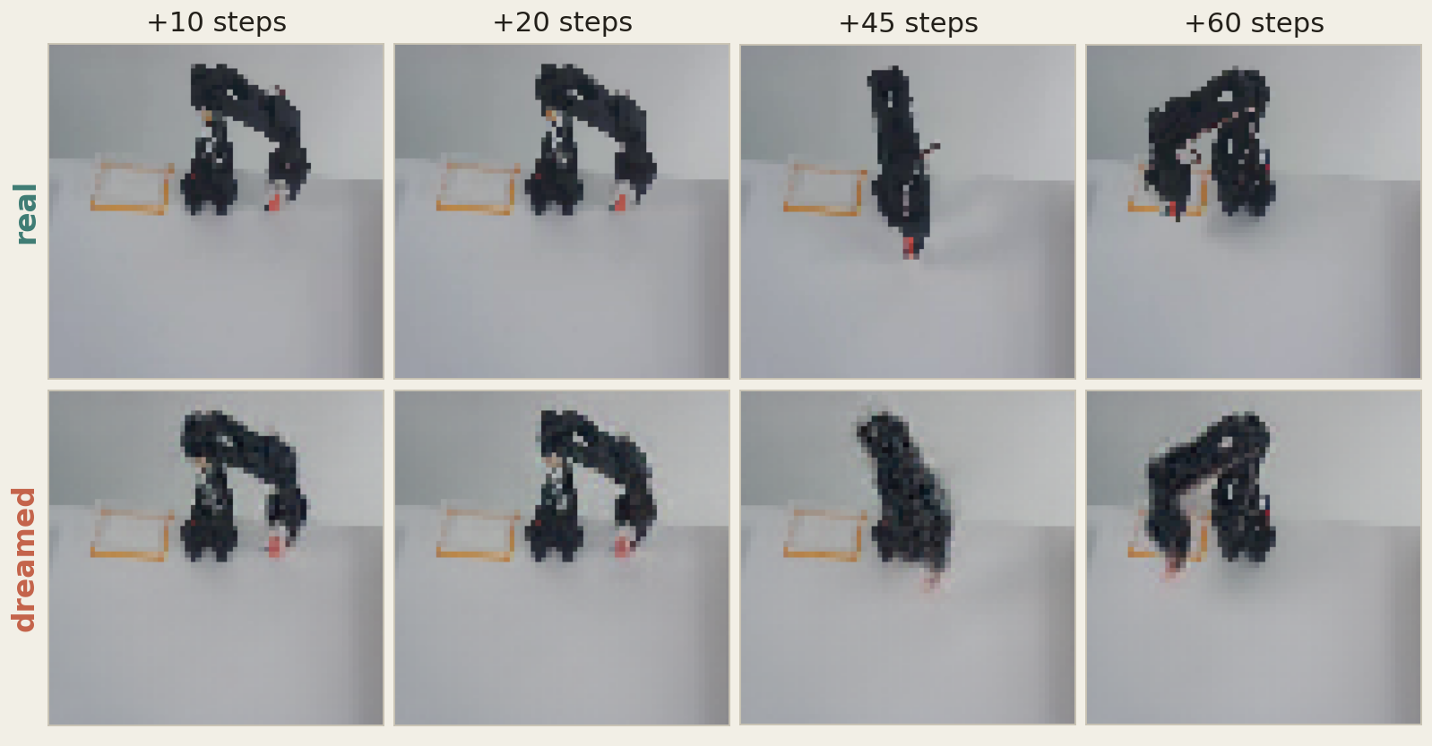
Lecture 4's imagination: correct — and soft. The blur is not undertraining. It is the shape of the latent.

Today we find out why, and the answer is not "train it longer." The blur is a structural consequence of two design choices we had never questioned: what the state is made of (a continuous vector) and how the model reads its own past (a recurrent summary). IRIS — the 2022 paper this pod opens up — flips both at once. To understand it honestly, we take the two choices apart, on text first, because a vocabulary is something you already understand and both ideas were proven on language.

Section 2: The Bottleneck, Measured

Strip a sequence model down to its bare job: take a news article, cover the next word, predict it. That is the entire task — and it is precisely what a world model does, with frames instead of words. The parallel we lean on all pod long: word ↔ frame, sentence ↔ episode, vocabulary ↔ ? — and the question mark is what this pod fills in.

There are two fundamentally different ways to read a sequence.

Idea one: carry a running summary. Read left to right, keep one fixed-size vector, update it at every word. This is a GRU — the machine that carried the robot's memory in Lecture 4. The appeal: reading word 1,000 costs exactly what reading word 1 costs, and memory never grows. The catch: everything the model will ever know about word 1 has to survive inside that one vector. Nothing else is kept.

Idea two: keep everything, and look back. The position doing the predicting forms a query ("I need a person's name"); every earlier word advertises a key ("I am a name", "I am a preposition"); strong matches hand over their value. That is attention — a weighted average of the past where the model picks the weights, and distance costs nothing.

Rather than argue, we measured. A newspaper-shaped passage names a minister in the first sentence, then N words of committee filler, then asks who resigned? The answer is always in the text; the only variable is how far back it sits — 4, 12, 24, 48, 96, or 160 words. Both models see identical data, budget, and size. With eight possible names, guessing blind scores 0.125.

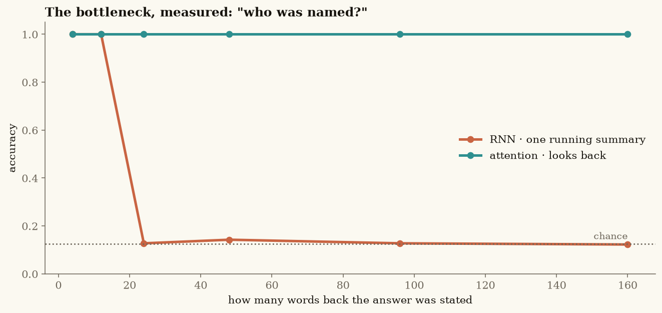
The bottleneck is not a metaphor — it is a cliff. The RNN is perfect at a 12-word gap and at chance by 24; attention holds at 1.00 all the way out to 160 words.

The result is sharper than we expected. The RNN is at 100% when the answer sits 12 words back — nothing wrong with a running summary as such. By a 24-word gap it scores 0.11 against a chance rate of 0.125, and it never recovers: 0.14, 0.13, 0.12 at 48, 96, and 160. The name did not fade gracefully; it was overwritten. A fixed-size memory does not degrade — it falls off a cliff. Attention, on the same data, stays at 1.00 all the way out to 160 words; inspect the trained model and the question token puts a quarter of its attention on a name 27 words back, having discovered where to look purely from being scored on the answer. This failure is exactly Lecture 4's gripper hiding the cube for fifteen frames.

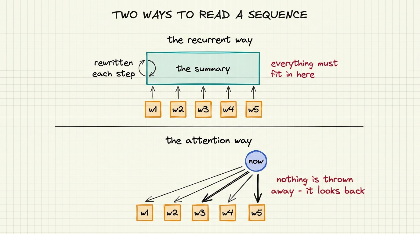
Compress and move on, or keep everything and choose. The recurrent way funnels the past into one box; the attention way keeps every word and selects.

Three consequences return at the end. Cost per step: recurrent is constant forever; attention grows with how much you keep. Fidelity: recurrent is lossy but free; attention is lossless but you pay rent every step. Training: recurrent is strictly sequential, while attention scores every position in parallel — which, more than anything, is why transformers scaled.

Notice what we have not changed yet: in both cases, the thing being passed around is still a bundle of continuous numbers.

Section 3: Points or Words — What a Latent Can Be

A latent is a short description of a thing, from which the thing can be rebuilt. Lecture 3 used 12 numbers for a Pong frame; Lecture 4 used 288 for a robot scene. We have only ever used one kind: continuous — real numbers, any value, arbitrarily fine. But there is a second kind: discrete — a symbol chosen from a finite list. Language works this way: a sentence is a sequence of choices from a vocabulary.

To see what each kind buys, we described the same corpus both ways: 2,041 real newsgroup posts across 6 topics, each turned into a 64-number vector (TF-IDF over an 8,000-word vocabulary, then SVD) and projected to 2D.

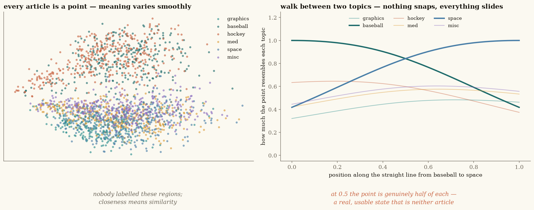
A continuous latent space: every article is a point, topics form regions nobody labelled, and you can walk from the baseball centre to the space centre and watch every topic score slide.

The continuous map has genuine virtues. Nearby means similar. The in-between places are real: an article about a hockey players' strike lands between sport and politics because it genuinely is between them. You can interpolate. The discrete description gives all of that up: a vocabulary can be enumerated — you can print the entire state space — but there is nothing between two of its entries.

So discrete looks strictly worse. Why choose it? Exactly one reason, and it is decisive. Ask a question with more than one right answer: "The match was cancelled because of the ____." Rain. Snow. A strike. All plausible, all different. A continuous model with a single Gaussian head must answer with a point — and under a squared-error loss, the safest point is the average of the possibilities. But the average of rain, snow, and strike is not a word. It is a location in the space where no word lives. Decode it, and you get a blur.

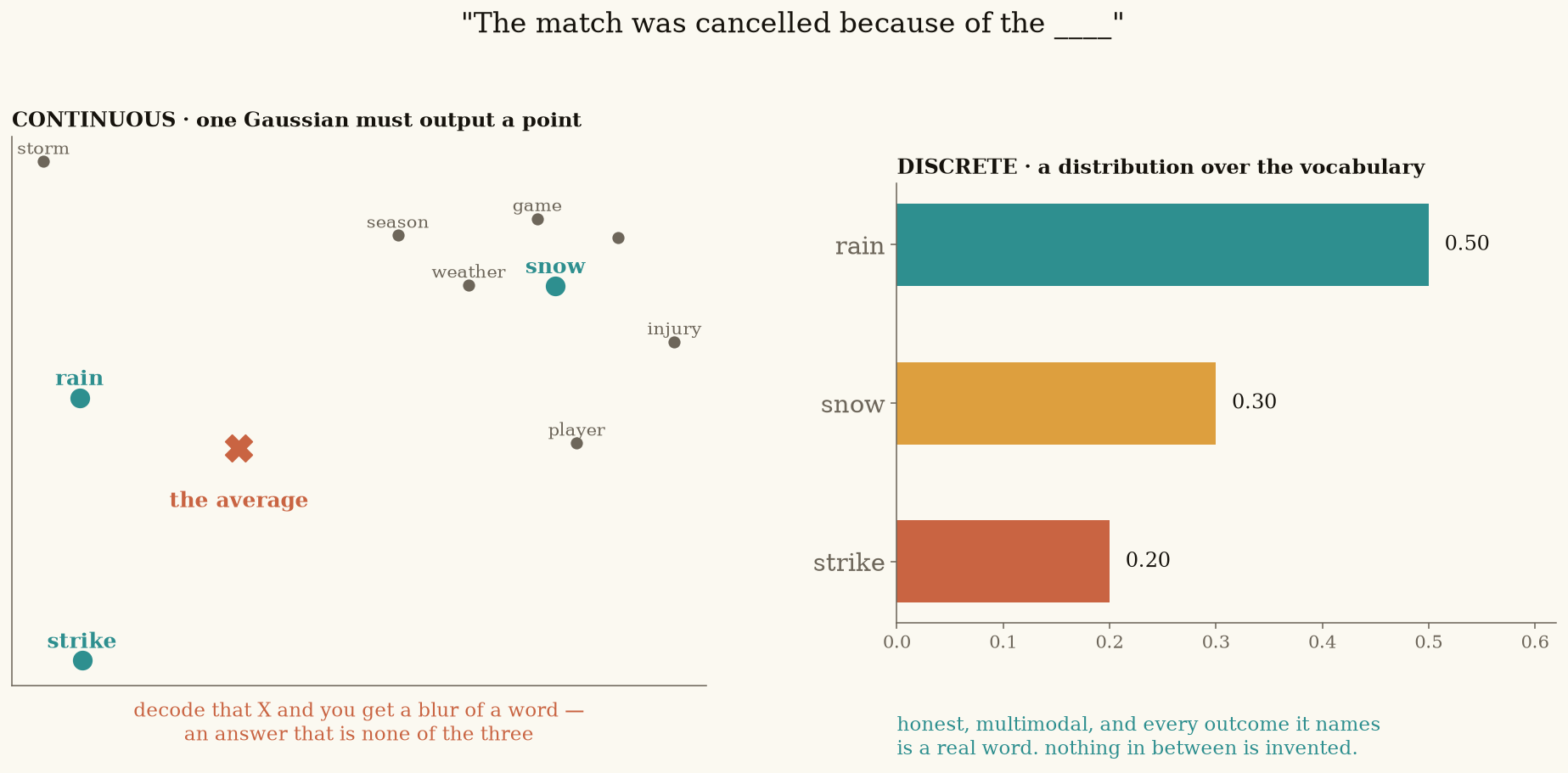
The pivotal difference: a single Gaussian must output a point, and the point between three words is not a word. A distribution over a vocabulary names only real options.

A distribution over a vocabulary, by contrast, can say "either this or that, and nothing in between" — natively. That is the whole trade: continuous wins when the world varies smoothly (arm positions, angles, velocities); discrete wins when the world makes choices (did the grasp catch or slip? did the platform appear or not?) — either-or events where the average is a lie.

The obvious objection: why not several Gaussians? That is a mixture density network — exactly what Ha and Schmidhuber used in the original World Models paper, and it genuinely works. But you must choose the number of modes in advance, and the world does not tell you the number. A vocabulary is a mixture with the number chosen for you: 512 "modes", one per dictionary entry, with the model deciding how many to use by how it spreads its probability — which is why the entire machinery of language modelling then applies unchanged.

And now we can name what happened in Lecture 4. Our latent was one Gaussian. Wherever the world could plausibly go two ways, the model had exactly one move: put the centre between them. The decoder faithfully painted the average — and an average of sharp frames is a soft frame. The blur was not a training failure; the model was doing precisely what we asked. The fix is a different kind of latent.

Which sets up the problem the next section must solve: text arrives with a vocabulary. A picture does not.

Section 4: Building a Vocabulary for Pixels

A 64×64 CoinRun frame is 12,288 raw numbers. There is no dictionary of "platform", "coin", "sky" hiding in a screenshot — so we have to invent one, and learn it from the frames themselves.

The trick is a fixed-size dictionary of vectors called the codebook: a list of, say, 512 vectors. To describe a patch of image, run it through an encoder, find the nearest codebook entry, and write down that entry's number. The patch is now a word. Encoder, snap-to-nearest, decoder — that is a VQ-VAE.

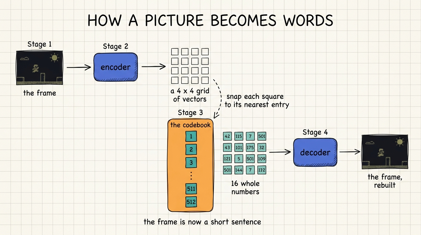
From 12,288 numbers down to sixteen: a 64×64 frame becomes a 4×4 grid of whole numbers — sixteen words drawn from a 512-word dictionary.

One deliberate choice matters enormously: the encoder produces a 4×4 grid, so each frame becomes sixteen words, not one. A single word per frame would need a dictionary entry for every possible scene — 512 entries would mean 512 possible frames in the whole game. With a grid, the words compose: this cell is sky, that one is ledge-edge, this one has the player on it. Sixteen slots with 512 choices each is an astronomically large space built from 512 reusable parts — exactly how language works. English does not have a word per sentence; it has ~50,000 words that combine. The frame becomes a short sentence, and now a language model can read it.

Training the tokenizer is a tug-of-war between two losses. Loss 1 spans the whole pipeline: the decoded frame must match the real one, pixel by pixel. Loss 2 spans one small gap: the chosen word's vector must stay near what the encoder actually produced, pulling from both ends — the codebook toward the encoder and the encoder toward its own dictionary. (In practice the codebook moves by an exponential moving average of the vectors assigned to each entry, standard since the original VQ-VAE paper.)

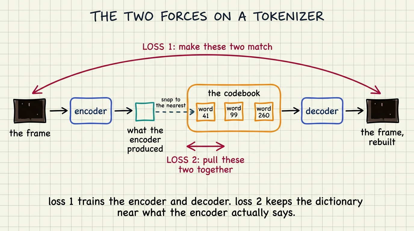
The two forces acting on a tokenizer: rebuild the frame, and keep the words near what the encoder actually said.

Two details decide whether this works at all. First, "snap to nearest" is a jump, and a jump has zero gradient — nothing upstream would ever learn. The fix is the straight-through estimator: use the snapped vector in the forward pass, and in the backward pass pretend the snap never happened. One line of code. Second, the classic silent failure: codebook collapse, where only a handful of entries ever get used — a 512-word dictionary in which the model only ever says three words. Reconstruction can still look fine, so you must measure it: track perplexity (roughly, how many words are really in use) and revive unused entries. We report our own numbers shortly rather than assume.

Section 5: IRIS — The World Model Becomes a Language Model

IRIS is three components, and the first two are trained separately, one after the other.

A tokenizer, trained first and then frozen. A VQ-VAE. In: one 64×64 frame. Out: 16 integers. It knows nothing about time, actions, or the future — purely a compressor, and once it is good it never changes again.

A dynamics model, trained second, on tokens only. A causal transformer. In: the last few frames as tokens, interleaved with the actions taken — the action is just a seventeenth token after each frame's sixteen. Out: a probability over the 512 words for the next token. It never sees a pixel.

And in the paper, an agent trained inside the dream. IRIS trains an actor-critic entirely on imagined rollouts. We stop before this — everything we build imagines; nothing yet acts.

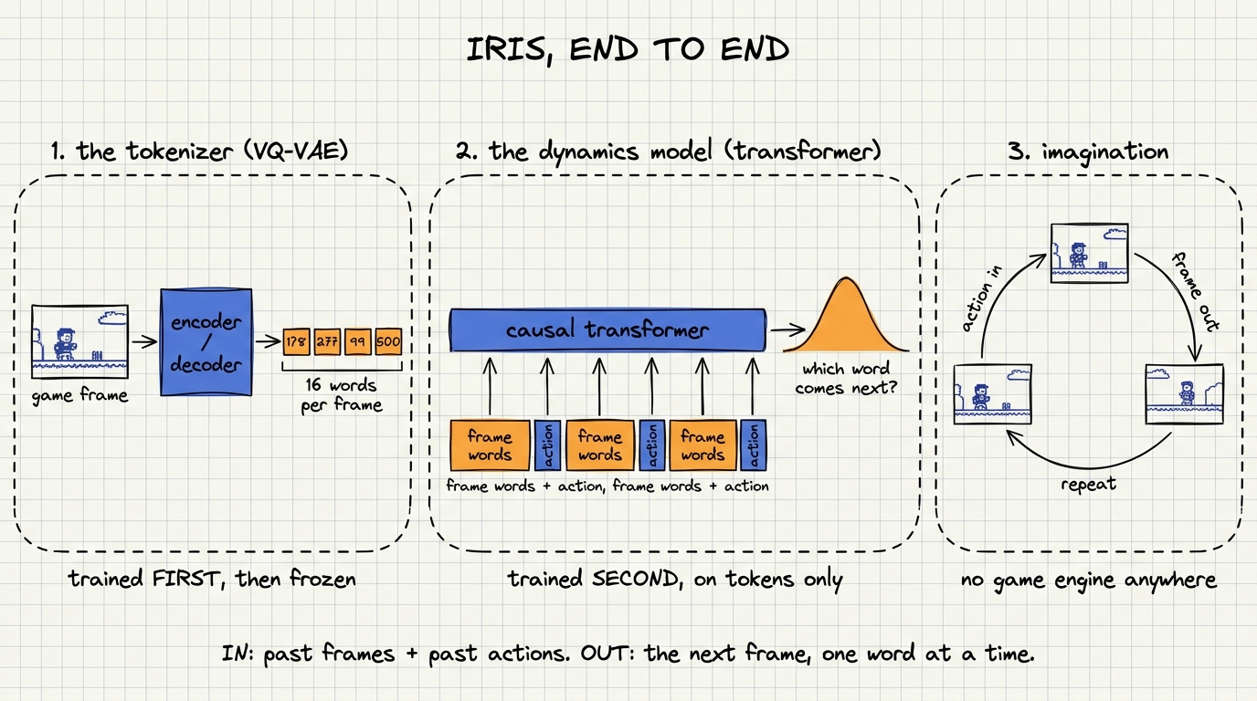
IRIS end to end: frames become tokens, actions become tokens, and a causal transformer predicts the next token — exactly how a language model writes the next word.

Why two stages? Because otherwise the vocabulary would move under your feet: if the tokenizer kept learning, word #99 would mean something different every few hundred steps, and the transformer would be modelling a language whose words keep changing meaning. Freezing the tokenizer turns stage two into pure language modelling — the whole dataset gets converted to integers once, and the transformer trains on a file of numbers without ever touching an image. That is exactly what we did: tokenizer for 20,000 steps, then the corpus tokenised once, then the transformer for 60,000 steps on the token file.

Step back and notice what IRIS changed: both of our assumptions at once. The latent became discrete — sixteen words per frame, so the model predicts a distribution over a vocabulary, with everything Section 3 said that buys. And the memory became attention — no hidden state carried between steps; the transformer looks back over the raw token history directly, the fix Section 2 measured. Once frames are tokens, a world model is a language model, and every trick from that world — sampling temperature, top-k, scaling laws — arrives for free.

One honest note: these are two independent choices, and IRIS flips both, which makes it easy to confuse which change did what. Every combination of {recurrent, attention} × {continuous, discrete} has been built, and all four corners are still in use today.

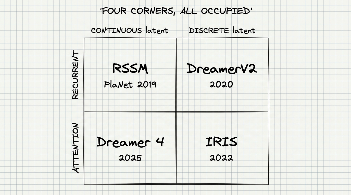
Two independent choices, and every combination has been built: the RSSM (recurrent + continuous), DreamerV2 (recurrent + discrete), IRIS (attention + discrete), and Dreamer 4 (attention + continuous).

The RSSM of Lecture 4 is recurrent + continuous. DreamerV2 kept the recurrent belt but swapped the Gaussian for categorical variables — proof the choices really are independent. IRIS took attention + discrete. And attention + continuous is Dreamer 4 — the corner people forget exists.

Section 6: Head to Head on CoinRun

Talk is cheap; we trained both. We generated 600 CoinRun episodes — 256,151 frames — with a random policy, and trained two world models on exactly the same data: Model A, an RSSM in Lecture 4's design (32 continuous state numbers, a GRU, a Gaussian latent, 5,364,035 parameters), and Model B, an IRIS-mini (16 words from a 512-word codebook, a causal transformer, 6,882,499 parameters). The two are matched on training wall-clock, land within 28% on parameters, and 40 held-out episodes were never seen by either. It is still not a perfectly controlled comparison — IRIS changes two things at once — and we flag that where it matters.

First: is the dictionary real? Codebook usage perplexity came out at 472 of a possible 512, with all 512 codes alive — no collapse. Reconstruction on held-out episodes: pixel MSE 0.00081. Twelve thousand numbers in, sixteen whole numbers out, and the game is still legible.

And now we can do something no continuous model permits: print the model's entire world.

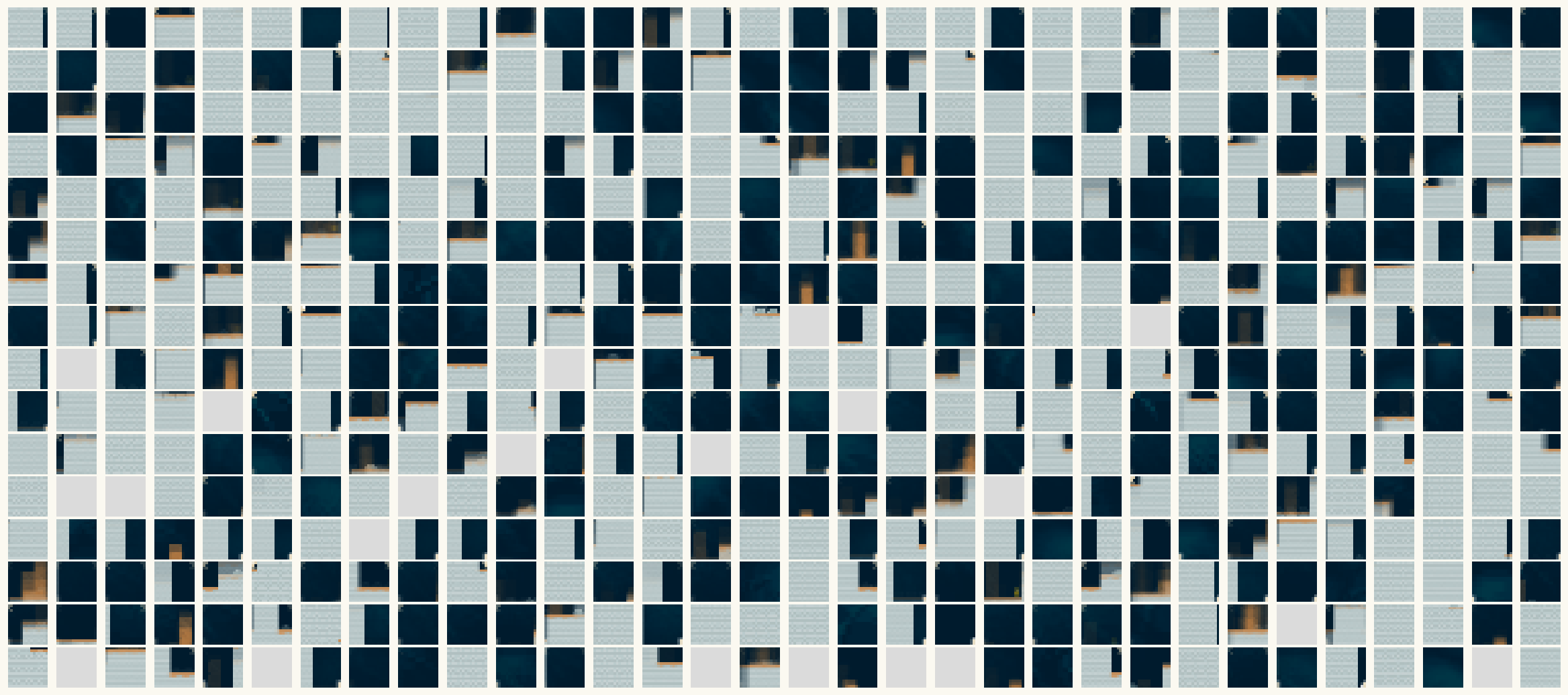
All 512 visual words this model invented for CoinRun — each square is one codebook word, shown as the average of the real 16×16 image patches assigned to it. Nobody labelled any of these.

Every frame this model will ever describe, dream, or predict is assembled from sixteen of these squares; there is nothing else in its world. That is Section 3's "enumerable" made completely literal — try printing a 32-dimensional Gaussian. (A methodological note: the model learns 512 vectors, not pictures. To draw them we ran 34,560 held-out patches through the tokenizer and averaged the real patches assigned to each word — 491 of the 512 appeared in that sample.)

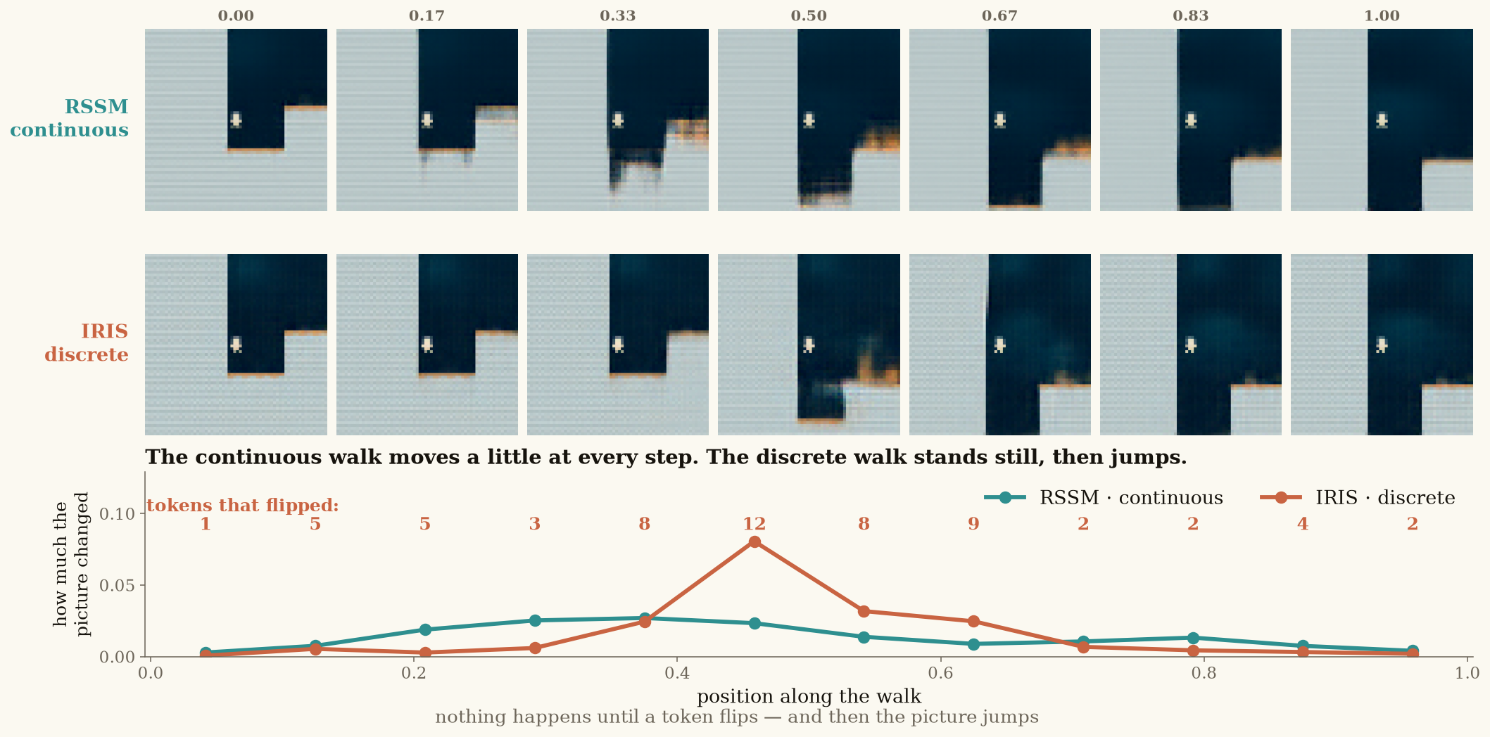
The two latent spaces behave exactly as the theory said. Walk between two frames inside each space and the continuous one morphs — every intermediate frame a genuine point in the RSSM's space, most of them scenes CoinRun could never produce — while the discrete one jumps from one combination of real words to another, because there is nothing in between to land on.

Walking between two frames inside each latent space: the continuous space passes through states that never occurred in the game; the discrete space can only ever land on real words.

And the headline question — did discreteness fix the blur? Section 3 predicted it: a categorical model cannot average two futures, so its dreams should be sharper, even when wrong. We measured edge sharpness on twelve imagined steps from the same context and actions: real footage 0.068, the RSSM 0.051, IRIS 0.067 (± 0.002 over 5 seeded rollouts) — 1.31× sharper. Note where each lands: the RSSM sits below the real game — too smooth, which is what averaging futures looks like — while IRIS sits essentially level with it.

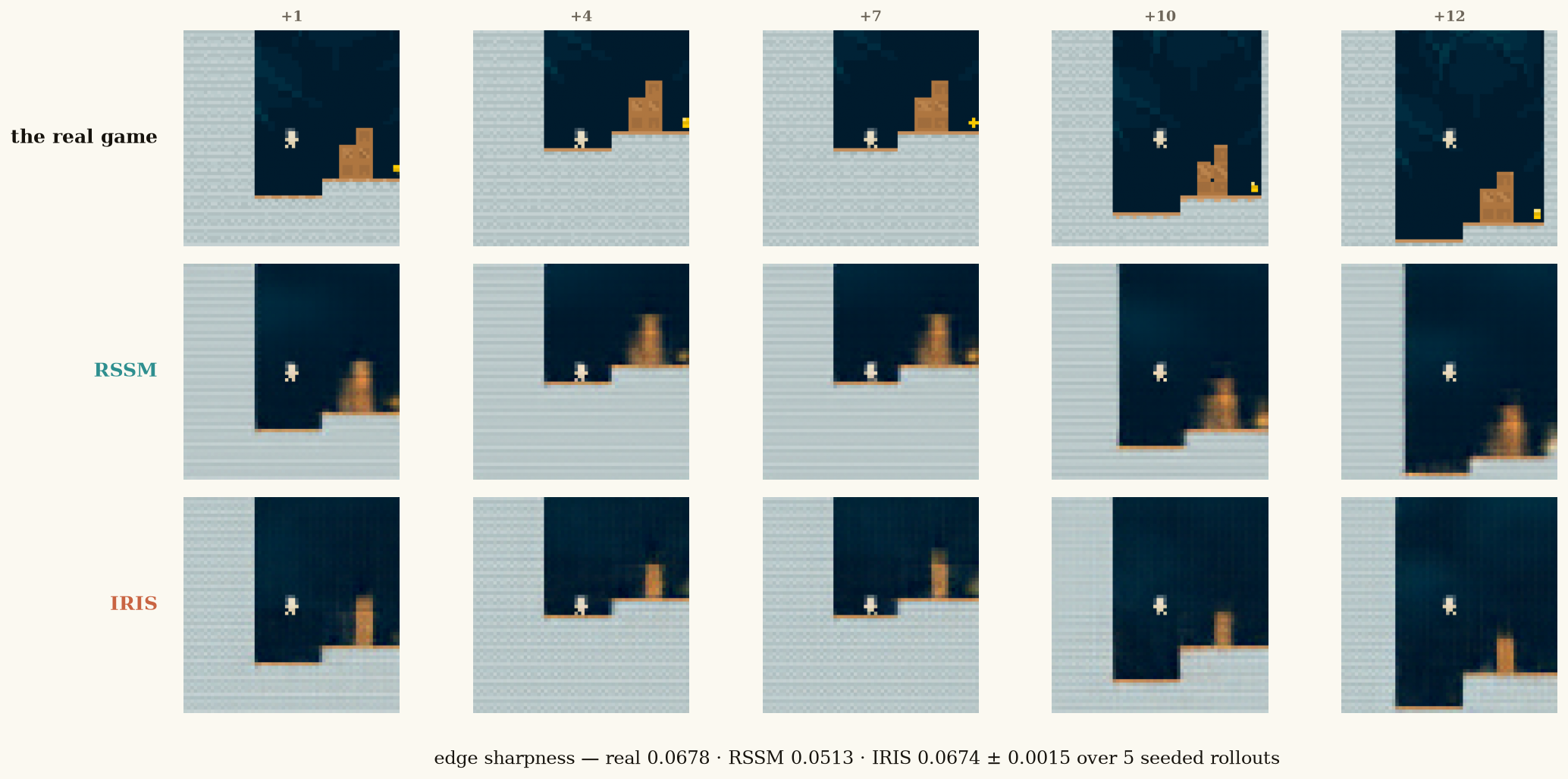
Twelve imagined steps, same context, same actions: what really happened, the RSSM's dream, and IRIS sampling tokens. Edge sharpness 0.068 / 0.051 / 0.067.

One distinction may be the most important sentence in this pod: sharp is not the same as correct. A token model can produce a crisp frame showing something that never happens; a Gaussian model produces a soft frame that is roughly right. Which failure you prefer depends entirely on what you will do with the dream.

The transformer's explicit memory also lets us ask a question the RSSM structurally cannot answer: how far back does it need to look? Because the past is kept as tokens, we can literally blank the oldest frames out and re-measure. One visible frame: cross-entropy 1.57 on the newest frame's tokens — the model is lost, because a single still cannot show which way the player is moving. Two frames: 0.099. Three: 0.019, and flat from there. On CoinRun the useful past is about three frames deep — an honest, slightly deflating result (a random policy on procedural levels creates few long-range dependencies), and exactly why we measured it instead of assuming. The RSSM has no such knob: there is no "back" to reveal.

Section 7: The Bill — What Each Design Costs

Now the price tag. We timed both models imagining futures on the same A10G GPU at batch size 1: the RSSM produced 5,783 imagined frames per second; IRIS produced 28. A factor of 206.

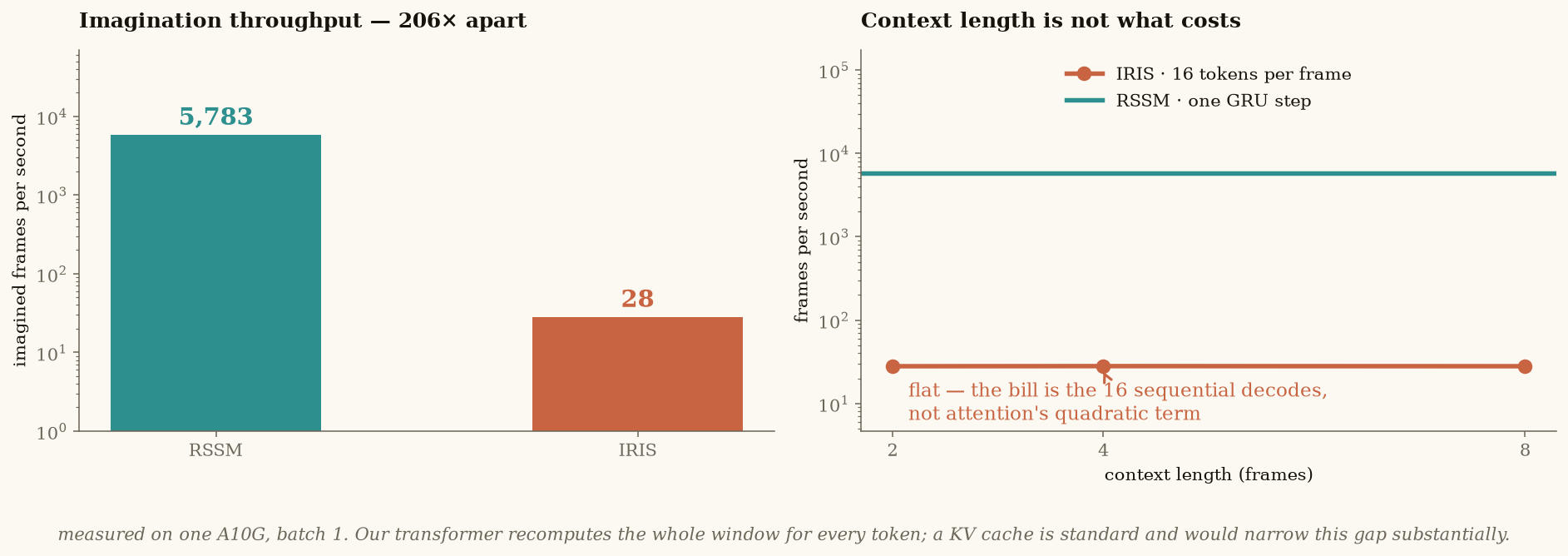
What each design costs to imagine with: 5,783 imagined frames per second for the RSSM against 28 for IRIS — and the transformer's throughput is flat across context sizes, so the gap is the sixteen sequential decodes, not attention's quadratic term.

Where does the gap come from? Not where the textbook says. The famous complaint about attention — quadratic cost in context length — is not what we measured: IRIS's throughput was flat at 27.9 / 28.0 / 27.9 frames per second across contexts of 2, 4, and 8 frames, because at 136 token positions the sequence is far too short for the quadratic term to bite. The real cost is that one imagined frame is sixteen sequential decodes: sixteen tokens, each sampled and written into the sequence before the next can be asked for — sixteen round trips through the whole transformer, against one small GRU step for the RSSM. (Honest headroom: our implementation recomputes the whole window for every token; a standard KV cache would narrow the gap substantially.)

So nobody won — and that is precisely why all four corners of the family tree are still occupied. Discreteness bought honest forks: a model that can say "either this or that" instead of painting the average. Attention bought perfect recall: no 24-word cliff, a past that is kept and inspectable. And the RSSM kept something neither has: imagination that costs the same at step 1,000 as at step 1 — and when an agent that plans wants to imagine thousands of futures, that constant cost stops being a detail and becomes the whole argument.

Four things to keep. A running summary has a cliff, not a slope. Continuous and discrete are good at opposite things — pick by asking whether your world varies smoothly or makes decisions. A vocabulary can be learned, not given — but always measure whether the model really uses it. And sharp is not the same as correct.

Next: this whole pod treated the transformer as a box that "predicts the next token." That is the what. In the next pod we open the box and trace a single picture-word through the entire trained network — in as an integer, out as a probability over 512 words — watching the embedding, the attention heads, and the residual stream do their work, with every number read straight out of our own model. The word goes in as 99. What comes out knows about the whole window. What happened in between is one of the best stories in deep learning.