The Good and Evil of the Key-Value Cache

How a clever trick that slashes computation silently moves the bottleneck somewhere else — and why your GPU feels it.

Let us start with a concrete situation. Imagine a language model sitting in front of a 2,000-token legal contract. A user has asked it to continue drafting the document, one word at a time. The model reads all 2,000 tokens, and now it is time to produce token number 2,001. Here is the uncomfortable truth about how a naive transformer inference loop actually works: to generate that single next word, the model re-reads every one of those 2,000 prior tokens, recomputes how each token relates to every other token through the attention mechanism, and produces a fresh set of intermediate representations — all from zero. Then, for token 2,002, it does the entire thing again. And again for 2,003. Every single generation step is a full replay of the entire context.

This is not a software bug. It is the natural consequence of how attention works, and it is the villain of our story. The cost of this approach grows so fast with sequence length that it quickly becomes catastrophically slow in practice. We will work through exactly why that is, in plain terms.

Then we will introduce the KV cache — and it is genuinely a brilliant fix. It collapses the repeated recomputation and makes generation dramatically faster. It is the hero.

But heroes always come with a price. Ours is no different. Once we see how the KV cache works, we will follow it all the way to the GPU's roofline model — a picture of how any computation is ultimately bounded by the hardware it runs on. And there, we will discover that the KV cache, while saving us an enormous amount of arithmetic, quietly creates a different kind of pressure. It taxes the memory system in a way that slides us into an uncomfortable region of the roofline, where the chip sits hungry, waiting for data. We will be honest about this tension, because understanding both sides is what lets engineers not just use these systems but actually improve them.

Let us begin with the hardware itself.

Section 1: The GPU Has Two Masters — VRAM and Bandwidth

A GPU is fundamentally a machine for doing a very large number of multiplications and additions very quickly. Modern GPUs used for deep learning can perform tens of trillions of such operations per second. That number is almost incomprehensible in its scale. If you handed a human a pencil and asked them to perform one multiplication per second, they would need millions of years to match what a GPU does in a single heartbeat.

But here is the catch. The GPU chip — the silicon that actually does the arithmetic — cannot operate on data it does not have in hand. Data lives in VRAM, which is the GPU's main memory. Before any computation can happen, that data must travel from VRAM across a physical data bus into the chip's local registers. And that journey has a speed limit. That speed limit is called memory bandwidth, and it is measured in bytes per second. On high-end hardware today, bandwidth typically sits somewhere between one and three terabytes per second — which sounds enormous, but we will shortly see how easy it is to saturate.

So we have two resources: the chip's arithmetic throughput (how many operations it can perform per second) and the memory bandwidth (how many bytes it can move per second from VRAM into the chip per second). These two numbers are fixed properties of the hardware. Every computation you run is ultimately constrained by whichever of these two resources runs out first.

This two-constraint picture has a name: the roofline model. Think of it as a simple plot. On one axis you measure the arithmetic intensity of your computation — roughly speaking, how many arithmetic operations you perform per byte of data you move. On the other axis you measure your achieved throughput. The roofline model says: if your arithmetic intensity is low, you are spending most of your time waiting for data to arrive, and your throughput is limited by bandwidth. If your arithmetic intensity is high, you have plenty of data to work with, and your throughput is limited by the chip's peak compute speed. The transition between these two regimes traces the shape of a roofline — sloping upward on the left, flat on the right.

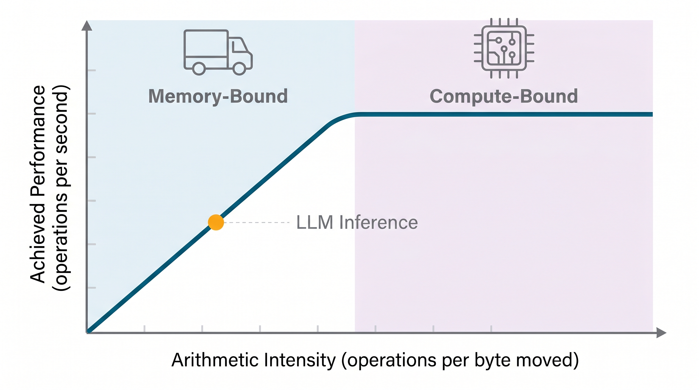
The roofline model shows LLM inference lives deep in the memory-bound regime.

The roofline model shows LLM inference lives deep in the memory-bound regime.

Let us ground this with a simple story. Imagine the GPU chip is a shipyard — a very fast one, capable of assembling one thousand units per second. Data arrives on delivery trucks from the warehouse (VRAM). Each truck delivers one hundred units per trip. No matter how fast the shipyard works, if it can only receive one hundred units per second, it will only assemble one hundred units per second. The shipyard sits idle for most of the day, waiting for the next truck. This is the memory-bound regime. The shipyard is not the bottleneck — the truck is.

Now flip it around. Suppose you flood the shipyard with deliveries — trucks arriving constantly, more than it can process. Now the truck is not the bottleneck; the shipyard's own assembly speed is. That is the compute-bound regime.

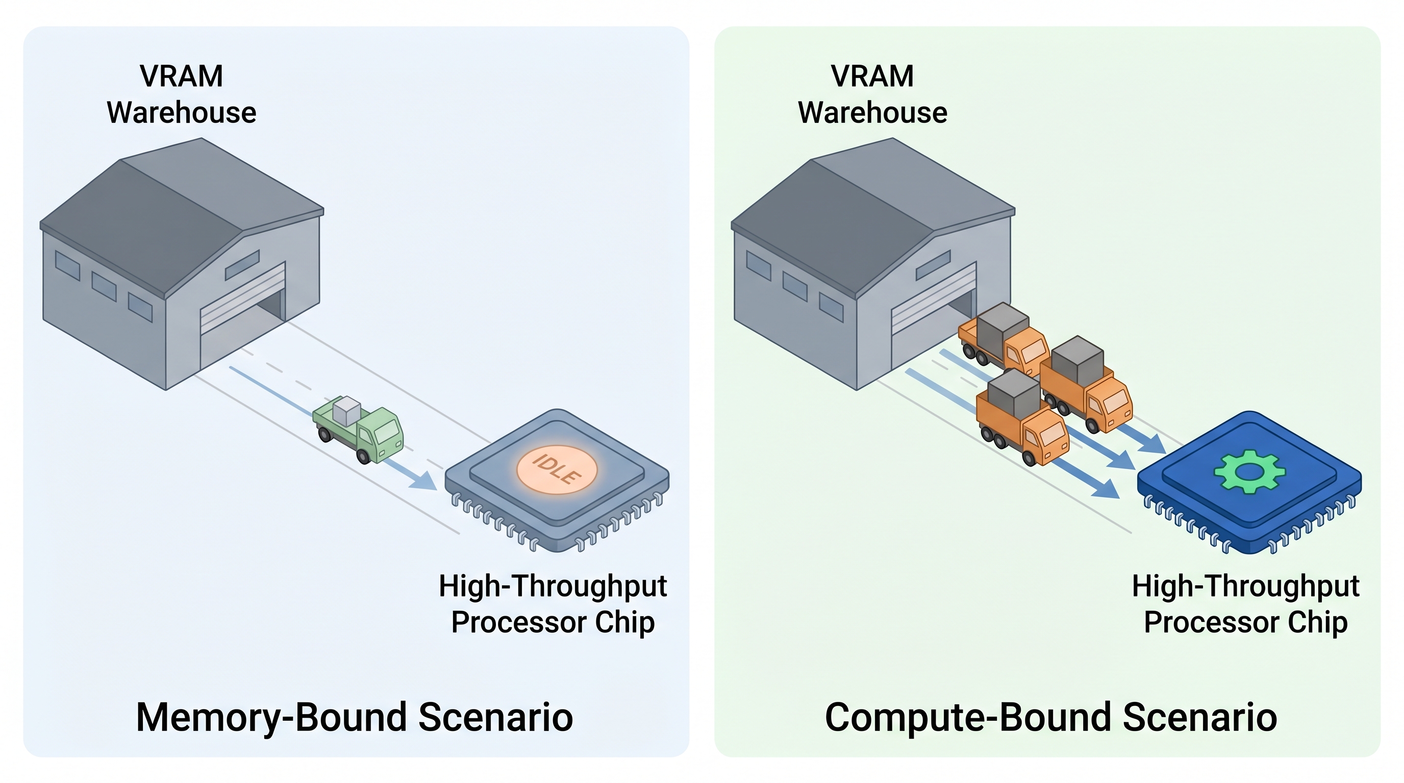
When data arrives slower than the chip can process it, the chip starves — that is memory-bound.

When data arrives slower than the chip can process it, the chip starves — that is memory-bound.

Where does LLM inference sit on this picture? Deep in the memory-bound regime. When a model generates tokens, the amount of arithmetic per byte of data is relatively small — we move model weights from VRAM, we perform some matrix multiplications, and then we wait for the next set of weights. The chip finishes its arithmetic quickly and then stalls, waiting for the truck. This is already the baseline situation for inference, before we even introduce the KV cache. Keep this picture in mind, because it is going to become the central lens through which we understand everything that follows.

Now the question is: what exactly does naive inference ask of this already-strained system?

Section 2: The Naive Inference Loop — An O(n³) Disaster

To understand what makes naive inference so expensive, we first need to understand what the attention mechanism is actually doing at each step. Let us do that in plain language, without any equations.

When a transformer processes a sequence of tokens, each token plays three roles simultaneously. First, it broadcasts a signal about what kind of information it is looking for — this is its query. Second, it advertises what kind of information it contains and can offer to others — this is its key. Third, it packages up the actual substance of what it contributes — this is its value. During attention, every token's query goes looking through all the other tokens' keys to find relevant ones. The more a query and a key resemble each other, the more attention gets paid. The values of the attended-to tokens then get blended together to form that token's output. This is how a word like "it" in a sentence finds the noun it refers to, even if that noun appeared fifty tokens earlier.

Now here is the important mechanical detail. Attention is not computed once and stored. In a naive transformer inference loop, every time you want to generate a new token, you run the entire attention computation from scratch over all tokens in the context. The new token's query must compare itself against every single prior token's key. To compute those keys and values, you must run every prior token through the key and value projection layers again.

This brings us to the cost question. Suppose you are generating token number 1,001 from a prompt of 1,000 tokens. At that step, attention runs over 1,000 tokens. For token 1,002, over 1,001 tokens. For token 1,100, over 1,100 tokens. Each step, the attention window grows by one. And recall that attention itself has a cost that scales with the square of the sequence length — every token must compare itself to every other token. When you add up the cost across all generation steps, and each step involves a growing quadratic cost, the total ends up scaling as the cube of the total sequence length.

Let us make this concrete. Suppose you are generating 100 new tokens from a 1,000-token prompt. At step one, you run attention over 1,000 tokens. That costs something proportional to 1,000 squared. At step two, 1,001 squared. By step 100, you are at 1,100 squared. Every single time, you recomputed the keys and values for all 1,000 original tokens — work you had already done in the previous step and simply thrown away. If generating 100 tokens takes a certain amount of time, generating 1,000 tokens does not take ten times longer — it takes far more, because each of those 1,000 steps is itself more expensive as the context window grows.

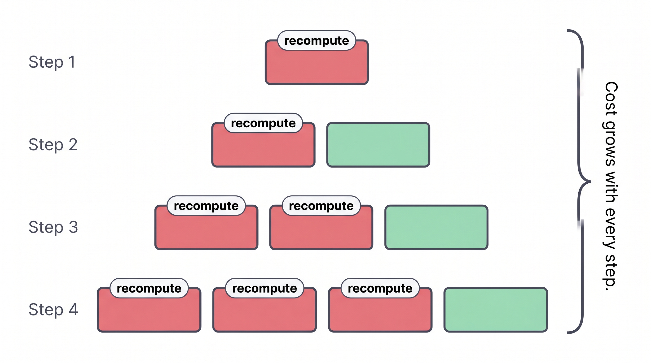
Without caching, every new token triggers full recomputation over all prior tokens.

Without caching, every new token triggers full recomputation over all prior tokens.

Think of it this way. Imagine you are a secretary taking meeting minutes. Every time a new attendee arrives, instead of just handing them the existing minutes, you re-interview every person who has ever been in the meeting, from the very beginning, and rewrite the entire document from scratch. For a meeting with ten people, that is annoying. For a meeting with two thousand people — and a legal contract that might be several thousand tokens — it is operationally impossible in any reasonable timeframe.

This is the naive inference loop. It is not that it produces wrong results — it produces perfectly correct results. It is just staggeringly wasteful. And the waste compounds. Every intermediate key and value tensor you computed in step one gets discarded before step two, even though those tensors are identical in both steps. You are re-doing the same work, over and over, for every single generation step.

This is exactly the problem the KV cache was designed to solve.

Section 3: Enter the KV Cache — The Hero We Needed

The key observation is deceptively simple. When you move from generating token 1,001 to generating token 1,002, what changes? The new query is different — it comes from the new token. But the keys and values for the previous 1,001 tokens? They are completely unchanged. A token's key and value are a function of that token and that token alone — they do not depend on what comes after. This means all that work we did in the previous step to compute those keys and values was not wasted — we just failed to save the result.

The KV cache is simply the act of saving that result. After computing the key and value representations for any token, we store them in a dedicated cache. On the next generation step, instead of recomputing keys and values for all prior tokens, we simply retrieve the stored ones and append the key and value for the one new token we just generated. The attention computation for the new query then just runs a single set of dot products against all the cached keys — one pass through the stored ledger — and we are done.

Think back to the meeting minutes analogy. In the naive case, we were re-interviewing everyone every time. Now, we keep a running notebook. When the meeting was at 1,000 people, we wrote down each person's entry. When person 1,001 arrives, we flip to the next blank page and add their entry. The notebook is the KV cache. No re-interviewing. No rewriting. The total work done to build the notebook across all steps is now proportional to the number of people, not the square of the number of people.

What does this mean for the cost of generation? Instead of each step paying a cost that grows with the square of the sequence length, each step now pays a roughly constant cost in terms of arithmetic — the cost of computing the new token's query, key, and value, plus one pass through the cached keys to do the attention dot products. The dot product pass still grows with the number of cached entries, but the key saving is that we are not recomputing all those cached entries anymore. Across the full generation of many tokens, the total work has dropped from something cubic in the sequence length to something quadratic — and the per-step wall-clock experience is dramatically faster.

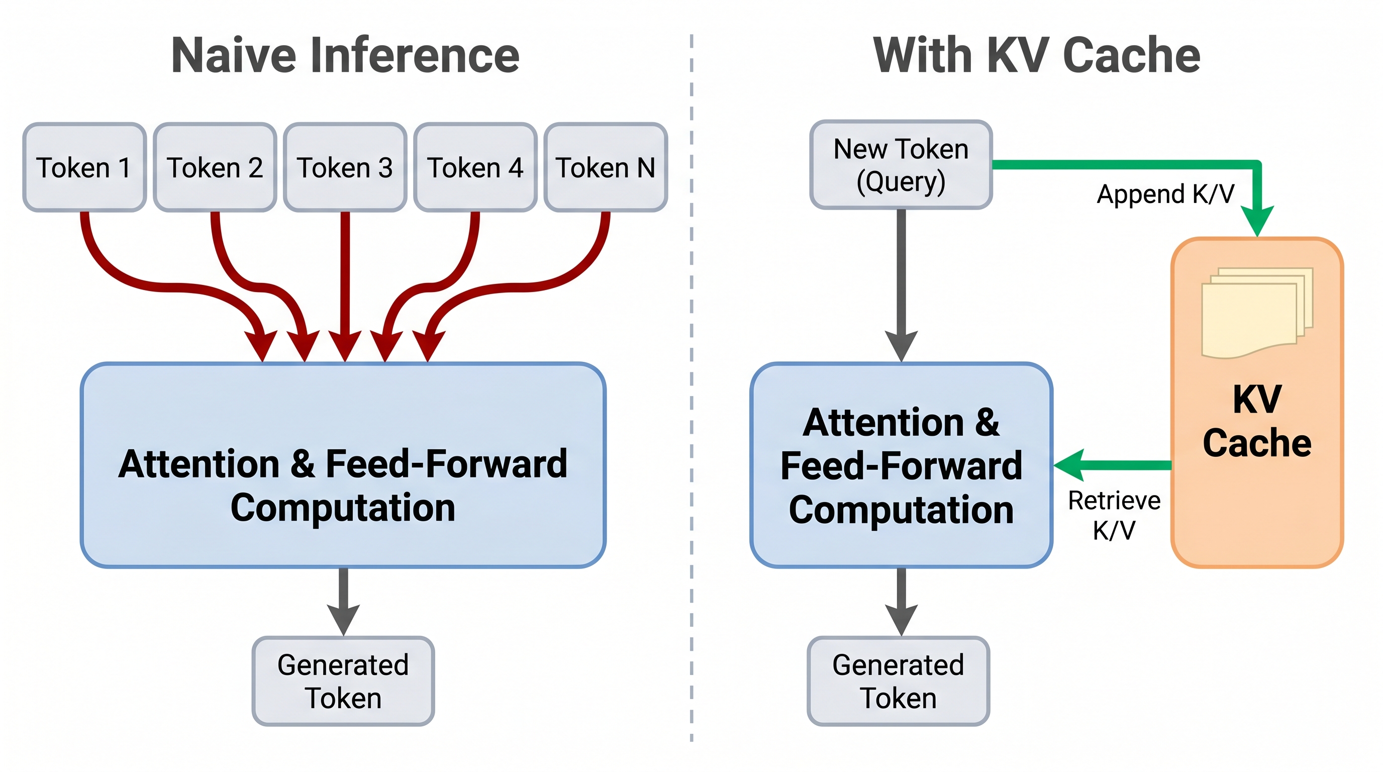
The KV cache stores past computations; each new step only adds one new entry.

The KV cache stores past computations; each new step only adds one new entry.

The wall-clock impact is real and measurable. If you run a language model generating long sequences and compare the two approaches, the gap is enormous. At short sequence lengths, the difference is modest. But as context length grows into the hundreds or thousands of tokens, naive inference slows down so dramatically that it becomes impractical. With the KV cache, generation remains fast enough to feel interactive even at context lengths that would have been completely infeasible otherwise. This is exactly what we want — and it is why every production inference system, without exception, uses the KV cache.

So the case for the KV cache is settled. It is necessary. It is brilliant. It is not optional.

But this is where most explanations stop, and where ours is just getting interesting. Because the KV cache does not just change how much arithmetic we do. It changes what the GPU is asked to carry — and that turns out to matter enormously.

Section 4: The Hidden Cost — What the KV Cache Does to Your GPU

Let us go back to the roofline model and think carefully about what the KV cache actually changes at the hardware level.

Before the KV cache, the naive inference loop was already sitting in the memory-bound regime, as we described. But it was memory-bound primarily because of model weights — to run the transformer's layers, you had to ferry those weights from VRAM into the chip repeatedly. There was also a substantial amount of arithmetic being done per byte moved, because attention was recomputing a full quadratic computation over all prior tokens.

Now, with the KV cache in place, consider what happens at each generation step. The model no longer recomputes keys and values for prior tokens. That computation is eliminated. Good — fewer operations. But those keys and values are now sitting in VRAM as a growing block of stored tensors. And to do the attention computation for the new query, every single one of them must be loaded from VRAM into the chip. Not just once — at every single generation step, the entire cache must be read out of memory and streamed through the chip so the new query can dot-product against it.

Here is what this means in terms of arithmetic intensity. We are moving a large and growing amount of data — the entire cache — in order to perform a relatively small amount of arithmetic: one set of dot products between the new query and all the cached keys. As the context grows longer, the cache grows, and the amount of data the truck must deliver at every step grows with it. Meanwhile, the arithmetic we do per step (one dot product pass) grows at the same rate, but the key point is that the ratio of arithmetic to bytes moved does not improve — and depending on model dimensions and batch sizes, it can actively worsen.

Recall the definition of arithmetic intensity from the roofline model: the ratio of operations performed to bytes transferred. When you reduce the operations (fewer FLOPs due to eliminating recomputation) but increase the bytes transferred (loading the full cache every step), you are decreasing arithmetic intensity. On the roofline plot, lower arithmetic intensity means you slide to the left. And sliding left in the memory-bound regime means you slide downward — lower achieved throughput.

The truck analogy captures this precisely. Before the KV cache, the ship (GPU chip) was doing redundant work, but the truck was also hauling a lot — it was busy shipping model weights and intermediate activations. After the KV cache, the ship finishes its arithmetic quickly and then sits there, idle, waiting for the truck to haul the entire cache archive from VRAM. The ship has less to do now — but it spends more time waiting, not less. We fixed the ship's redundancy problem, and in doing so, we handed the truck a bigger job.

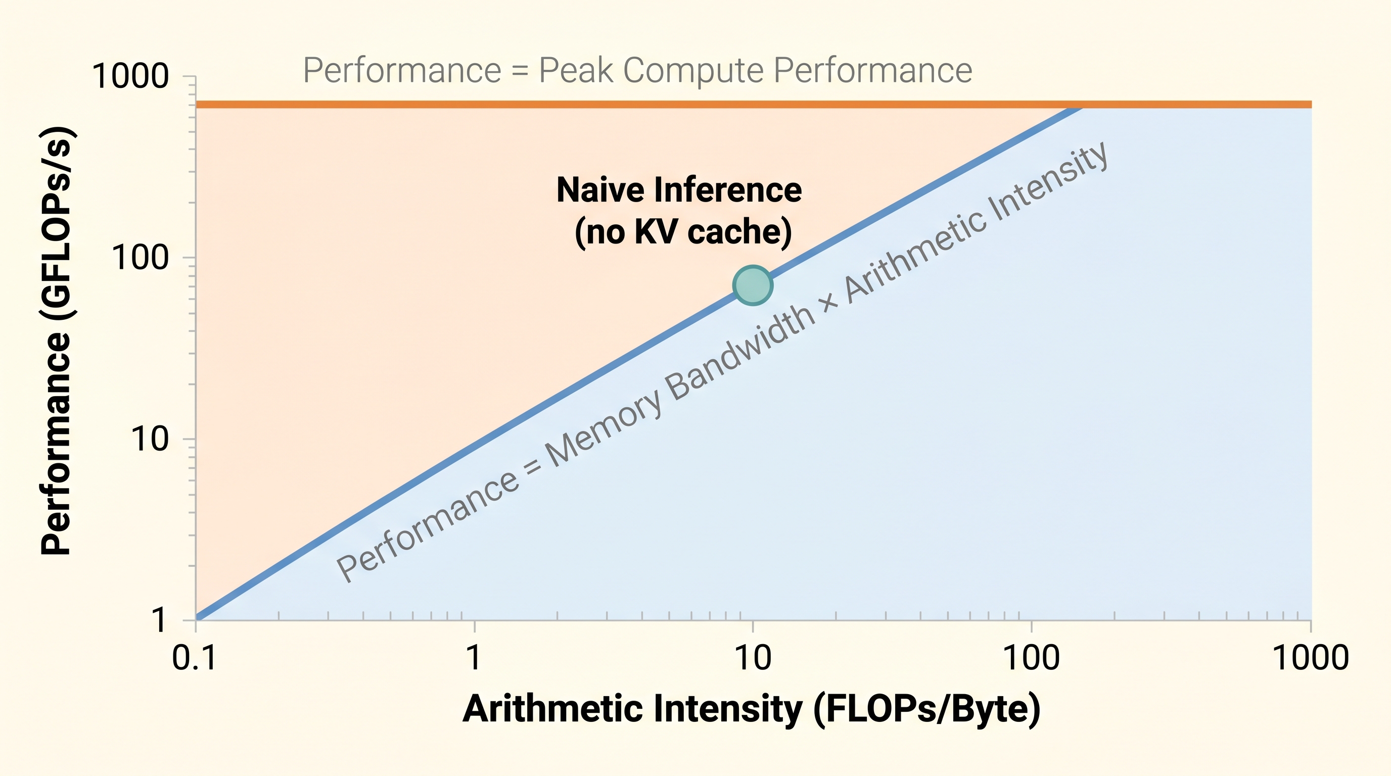
KV cache lowers arithmetic intensity, sliding inference deeper into memory-bound territory.

KV cache lowers arithmetic intensity, sliding inference deeper into memory-bound territory.

Let us ground this with some rough numbers to make it feel real. A typical large language model running in 16-bit floating point precision, processing a sequence of 4,096 tokens, across all attention layers and all heads, might accumulate a KV cache that weighs several gigabytes. On a high-end GPU with a memory bandwidth of around 2 terabytes per second, loading several gigabytes takes on the order of a millisecond or more per generation step. And this is not a one-time cost — it happens at every single token generation step. Across a response of a thousand tokens, those milliseconds accumulate. And as the context window grows, the cache grows with it.

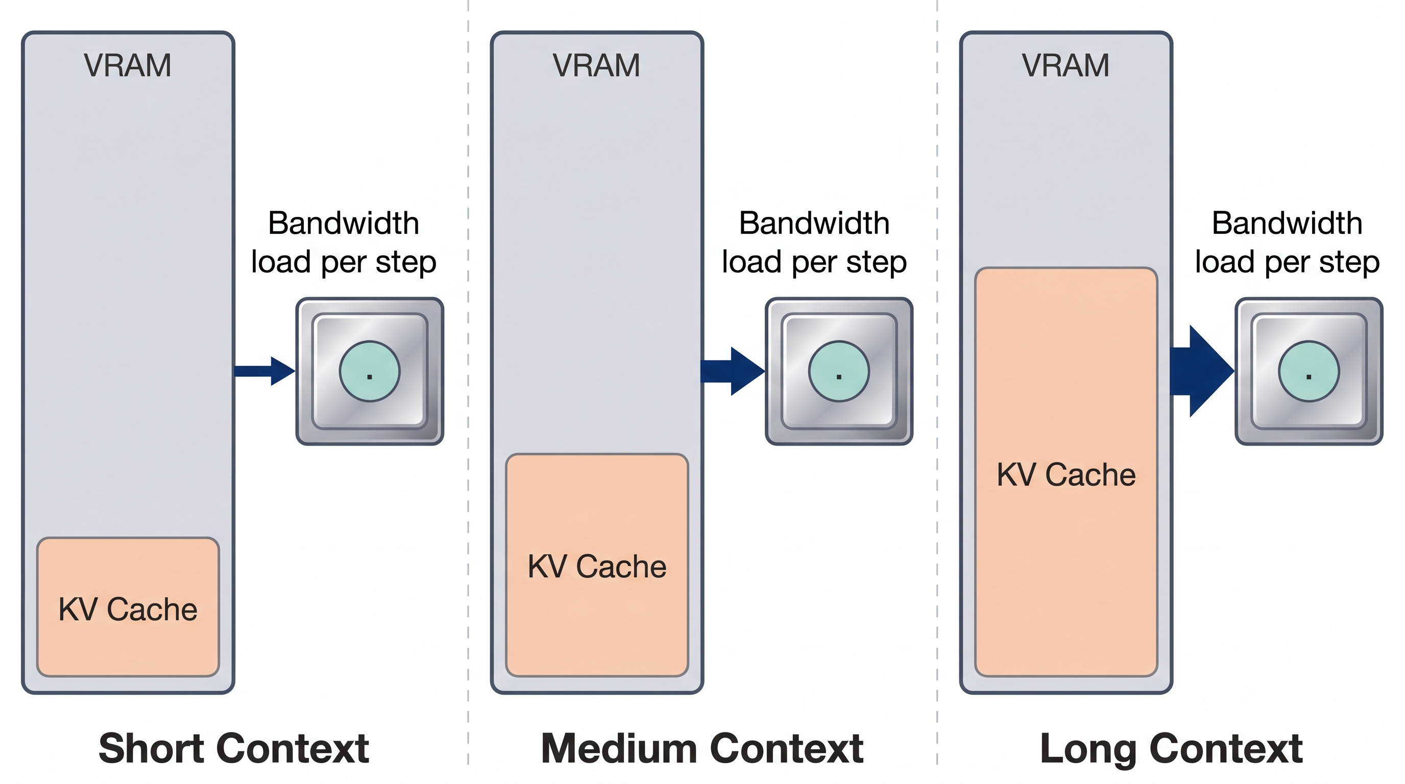
As context grows, cache bandwidth load increases while per-step arithmetic stays constant.

As context grows, cache bandwidth load increases while per-step arithmetic stays constant.

This is the irony at the heart of the KV cache. It is one of those interventions that solves a very real problem and simultaneously creates a quieter, harder-to-see problem. The FLOP savings are obvious and immediate — you can measure them directly. The bandwidth tax is subtler, because it shows up not as wrong answers but as a gradual degradation of throughput as sequences get longer. Engineers who only look at FLOP counts will think the KV cache is an unambiguous win. Engineers who look at the roofline will see the full picture.

So where does this leave us? The KV cache is not evil in the sense of being avoidable. There is no realistic alternative — the cubic scaling of naive inference is simply not acceptable. But the KV cache is a necessary evil in the precise sense that it replaces one form of inefficiency with another, quieter form. And the community has had to develop a whole family of techniques to manage the consequences.

Section 5: Living With the Necessary Evil — GQA, Quantization, and the Bandwidth Fight

Once you understand that the KV cache's core problem is memory bandwidth — the truck having too much to carry — the design space for solutions becomes clear. You either make the cache smaller, or you make the cache denser (more information per byte). Every major technique in this space is doing one of those two things.

Let us start with the most direct approach: making the cache smaller by redesigning how attention heads work.

In standard multi-head attention, every attention head has its own set of keys and values. If a model has 32 attention heads, then for every token in the context, you store 32 separate key vectors and 32 separate value vectors. All 32 sets get loaded from VRAM at every generation step. This is the baseline.

Grouped Query Attention, or GQA, questions the necessity of that arrangement. What if multiple query heads shared the same set of keys and values? Instead of 32 independent key-value pairs, you might have 8 groups of 4 query heads each, with each group sharing one key-value pair. Now you only need to store and load 8 sets of keys and values rather than 32. The cache is four times smaller. The truck hauls four times less. On the roofline, we have reduced the denominator — fewer bytes transferred — which means arithmetic intensity rises and we slide back to the right.

Multi-Query Attention takes this to the logical extreme: all query heads share a single key-value pair. The cache shrinks to a minimum. In practice, researchers have found that GQA hits a sweet spot — sharing enough to drastically reduce cache size without noticeably harming the quality of the attention computation. Most modern large language models, including the LLaMA family and many others, have adopted GQA precisely for this reason.

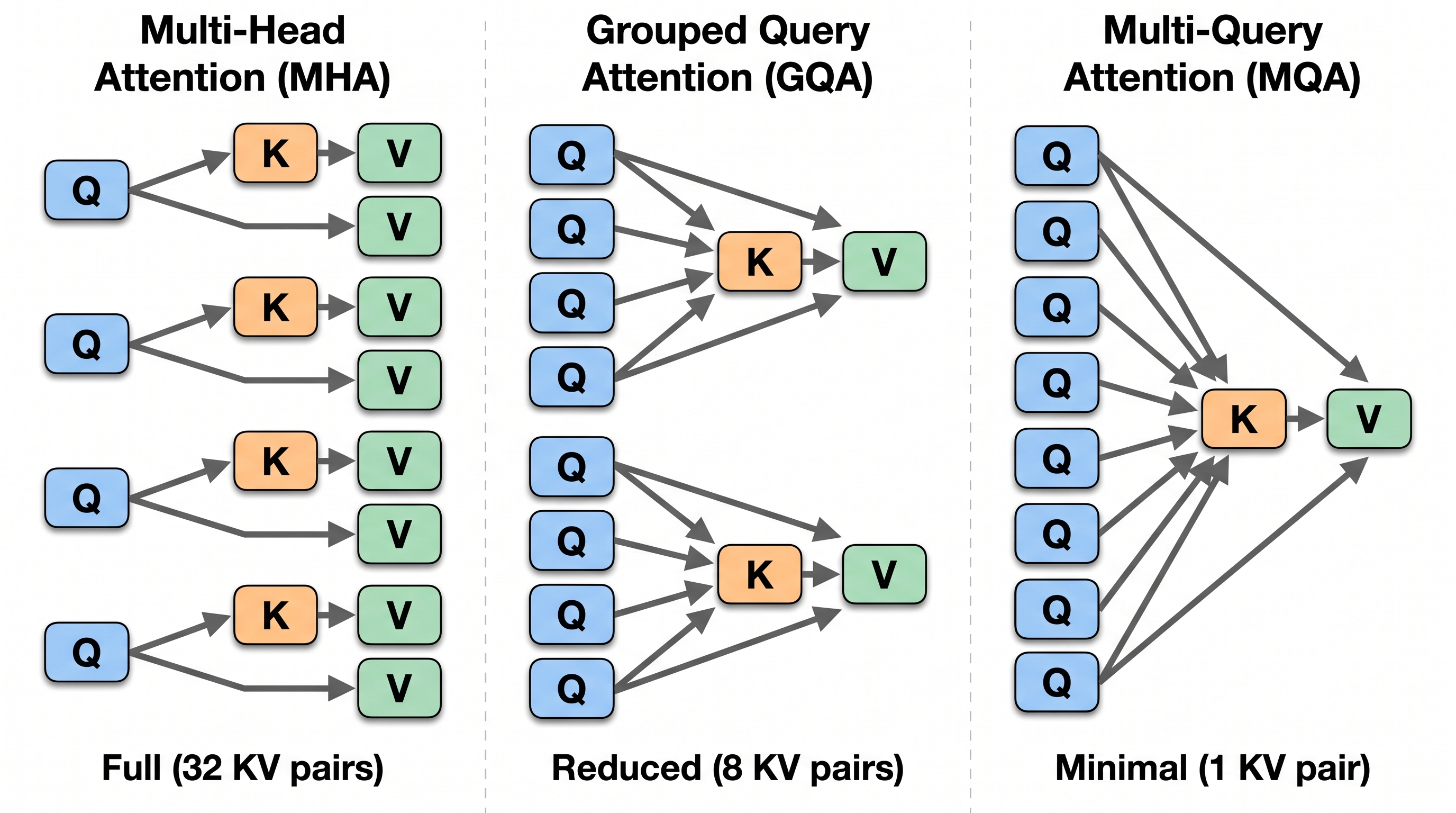
GQA and MQA shrink the KV cache by sharing key-value heads across queries.

GQA and MQA shrink the KV cache by sharing key-value heads across queries.

Now let us consider the second major approach: making the cache denser through quantization.

In standard operation, the cached keys and values are stored in 16-bit floating point format — two bytes per number. If instead we store them in 8-bit integers, we cut the cache size in half. In 4-bit integers, we cut it by another factor of two. Fewer bytes means the truck hauls less, arithmetic intensity rises, and we move right on the roofline.

KV cache quantization is appealing because it does not require any architectural change. You can take an existing model, quantize its KV cache, and immediately reduce the bandwidth pressure. Libraries like vLLM and frameworks like TensorRT-LLM have made this a standard option. The cost, of course, is potential accuracy loss — representing numbers in fewer bits means you can no longer represent them as precisely. Whether this accuracy loss matters depends on how sensitive the particular model and task are to small errors in the cached representations.

There is also a separate but related memory management concern addressed by techniques like paged attention, used in vLLM. This addresses not the bandwidth issue but the fragmentation problem — the fact that allocating memory for variable-length KV caches leads to wasted VRAM in the same way that a fragmented hard drive wastes space. Paged attention borrows the idea of virtual memory paging from operating systems and applies it to KV cache allocation, making memory usage much more efficient. This is an important technique, though it targets a different dimension of the problem than bandwidth.

All of these approaches — GQA, MQA, quantization, paged attention — are responses to the same underlying reality: the KV cache is a bandwidth consumer, and left unchecked, that consumption becomes the dominant constraint on how fast language models can generate.

But there is a subtler problem lurking inside KV cache quantization that none of these approaches fully address. It is not about how many bits you use to store the cache. It is about whether those bits are actually carrying useful information. And fixing that is where we arrive at TurboQuant.

Section 6: TurboQuant — Rotating Your Way to Better Cache Compression

Let us think carefully about what quantization actually does. When you quantize a vector — a list of numbers — you are replacing each number with the nearest value on a fixed grid. If you have 4-bit quantization, that grid has 16 levels. Those 16 levels must span the full range of the vector from its smallest to its largest value. Everything in between gets rounded to the nearest grid line.

This works well when the values in your vector are spread out reasonably evenly across their range. But attention keys and values in transformer models are not like that. They tend to be spiky. A typical key vector might have one or two components that are very large — close to the maximum value — and many other components that are tiny, clustered near zero. The spikes dominate the dynamic range, and the small components get crushed.

Here is the specific problem. Your 4-bit quantization grid must span the full range from the tiny values up to the spike. With 16 levels covering that entire range, each level covers a wide interval. The spike sits comfortably in its own level at the top — fine. But all the small components, which were actually carrying subtle information, are so close together relative to the full range that they all map to the same bottom level. They all become zero. You have just erased all the subtle information that was encoded in those small components.

The resulting quantized vector is essentially a one-hot vector — a spike at one position and zeros everywhere else. A one-hot vector over eight dimensions carries almost no real information. You spent 4 bits times 8 dimensions to store it, but the effective information content is a fraction of that. The bits are wasted.

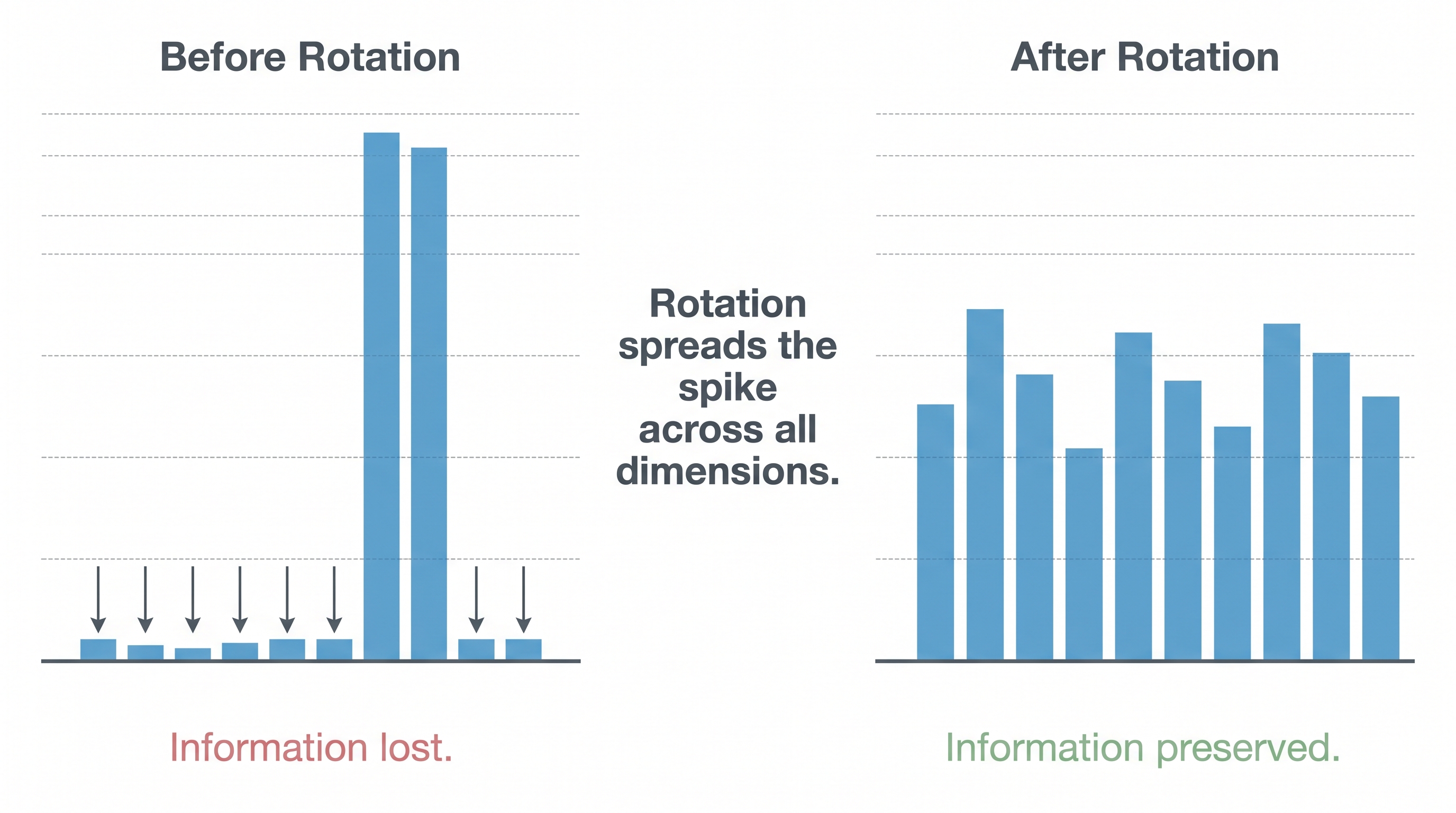
Rotating spiky vectors before quantization prevents small components from collapsing to zero.

Rotating spiky vectors before quantization prevents small components from collapsing to zero.

TurboQuant's answer to this is one of those ideas that sounds almost too simple when you first hear it. Before quantizing a key or value vector, rotate it. Apply a random rotation to the vector so that the large spike gets spread out across all dimensions. After the rotation, instead of one enormous component and many tiny ones, you have all components at roughly equal magnitude. Now the quantization grid does not have to waste most of its 16 levels representing a useless range that only the spike occupies. Every level gets used. Every component of the vector maps to a meaningfully distinct grid position. The bits carry real information.

Then, when you retrieve the quantized vector from the cache to use it in the attention computation, you first dequantize it and then rotate it back. The reverse rotation reconstructs the original vector as faithfully as the quantization precision allows — but now that reconstruction is much more faithful, because the quantization step did not throw away the small components.

Think about it in terms of packing luggage for the truck. In the unrotated case, you have one enormous suitcase (the spike) and seven nearly empty ones (the small components). The truck hauls eight suitcases, but seven of them are essentially empty — wasted capacity. After rotation, you redistribute the luggage evenly. Now all eight suitcases are packed efficiently. The truck hauls the same number of suitcases, but now each one is actually full. The information density per byte transferred goes up.

The rotation itself is just a matrix operation — the same rotation matrix is applied to all vectors, it does not need to be learned, and it is cheap to apply relative to the cost of the attention computation itself. The key insight is that a random rotation is, in a precise mathematical sense, an information-preserving transformation — it shuffles the values around without destroying any of the relationships between them. The fundamental information content of the vector is unchanged; only its distribution across dimensions is reshuffled. And that reshuffling happens to make the quantization grid fit the data much better.

The connection back to our central story is direct. Better quantization means fewer bytes needed to represent the same information. Fewer bytes in the cache means the truck hauls less at each generation step. Less data transferred means arithmetic intensity goes up. Arithmetic intensity going up means we slide right on the roofline, back toward the balanced operating point. TurboQuant is, at its core, a roofline optimization — it is trying to claw back the arithmetic intensity that the KV cache took from us.

This is exactly what we want.

The Full Picture

Let us step back and trace the arc of what we have built together.

We began with a language model asked to continue a long document, one token at a time. The naive approach — re-running the full attention computation from scratch at every step — scales disastrously as the sequence grows, accumulating a total cost that behaves cubically with sequence length. For long contexts, this is not just slow — it is effectively impossible at production scale.

The KV cache enters as the essential fix. By storing the key and value representations of all prior tokens and simply appending the new token's entries at each step, we eliminate the redundant recomputation. Per-step generation goes from a growing quadratic cost to something far more manageable. Wall-clock time drops dramatically. The KV cache is not optional — it is the foundational technique that makes interactive generation with long contexts possible at all.

But we followed the KV cache further than most treatments do. We took it to the roofline model, the hardware-level picture that bounds what any computation can achieve on a real GPU. And there, we found the hidden cost. By reducing FLOPs but massively increasing the amount of data that must be loaded from VRAM at every generation step, the KV cache decreases arithmetic intensity. It slides us further left and downward on the roofline — deeper into memory-bound territory — making the bandwidth bottleneck more severe, not less. We fixed the ship's redundancy problem and gave the truck a much heavier load.

This insight motivates the entire family of KV cache optimization techniques: Grouped Query Attention and Multi-Query Attention shrink the cache by sharing key-value pairs across heads; KV cache quantization reduces the bytes-per-entry by representing cached values in lower precision; paged attention manages the memory fragmentation that comes from variable-length caches. And at the frontier, TurboQuant addresses the subtle quality problem within quantization — the spiky distribution of key and value vectors that causes naive quantization to waste most of its bits on empty dynamic range — by applying a random rotation before quantizing and rotating back after dequantizing. Each of these techniques, in its own way, is trying to push arithmetic intensity back to the right on the roofline.

The KV cache is one of those engineering decisions that is simultaneously obviously necessary and quietly costly. You cannot build a production language model inference system without it. But if you treat it as a pure win — if you only look at the FLOP savings and ignore the bandwidth tax — you will be confused about why your GPU throughput degrades as contexts grow, why your hardware is not nearly as utilized as the FLOP counts suggest it should be, and why techniques like GQA and KV quantization exist at all.

Understanding both sides — the computation saved and the bandwidth consumed — is what separates engineers who use these systems from engineers who can genuinely improve them. The roofline model is the lens that makes both sides visible at once. Keep it in mind every time someone shows you a speedup in FLOPs. Always ask: but what happened to the truck?

Where the field went next: MLA and sparse attention

Everything above treats the KV cache as a fact of life to be managed — quantized, paged, grouped. The frontier labs asked a sharper question: what if the cache itself could be smaller by design? Two answers now dominate, and a reader of this pod — this section exists because one of you asked for it — should know both.

Multi-Head Latent Attention (MLA) is DeepSeek's answer. Instead of caching full keys and values per head, MLA caches a single low-rank latent vector per token and reconstructs the per-head keys and values from it on the fly. The cache shrinks by an order of magnitude while quality holds, because the latent is trained end-to-end rather than compressed after the fact. It is the reason DeepSeek's models serve long contexts so cheaply — and it is exactly the trade this pod taught you to see: a little extra compute (the reconstruction) purchased with a huge saving in memory bandwidth. The truck carries less; the forklift works slightly harder.

Sparse attention attacks the other axis: not how much each token costs to cache, but how many tokens attention has to read. If each query attends to a selected subset — recent tokens, a few global anchors, retrieved blocks — the bandwidth bill for million-token contexts stops scaling with the full sequence. DeepSeek's sparse attention makes the selection learned rather than fixed, which is what finally made the approach competitive in quality.

We teach both from scratch, weights and all:

If you finish this pod and go straight into those two, you will have walked the actual line of thought the field walked: cache everything → cache smarter → cache less by design.